Chapter 23: How Can Gaussian Snapshots Become Continuous Paths?—Continuous Modifications, Gaussian Processes and Wiener Measure

An instrument records positions at finitely many times. Increasing its sampling frequency makes the record denser, but does not prove what happened between observations. For random motion, more is missing than a few numerical positions: we must know whether all these readings can be realized by one continuous curve.

The Gaussian increments and covariance kernel of Chapter 4 are already quite specific. We now treat them as requirements to be fulfilled, rather than descriptions of a curve whose existence has been granted. Fulfilling them requires separating three tasks: specifying the laws of finite observations, choosing a version of a process, and putting probability on a space of continuous functions.

23.1 The same photographs need not make the same film

Simplify the motion as far as possible: every observation should return zero. The zero process satisfies this requirement. Chapter 8 gave another realization: choose U uniformly in (0,1), and change the value to one only at this random time.

The probability of hitting U at any fixed finite collection of times is zero. The processes therefore have identical finite-dimensional distributions. Yet every path of Y has an isolated spike, whereas X has continuous paths. This does not contradict the extension uniqueness in Chapter 8: that uniqueness concerns distributions on the coordinate event system, not arbitrary path properties whose measurability has not been established.

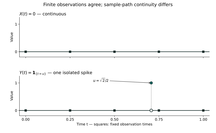
On one probability space, two processes are modifications of each other if Xₜ=Yₜ almost surely for each fixed t. They are indistinguishable if there is one measurable set of probability one on which equality holds for every t. The quantifiers cannot be interchanged. The example gives modifications that are not indistinguishable. If both modifications have continuous paths, intersect the equality events at countably many dense times and extend by continuity; they are then indistinguishable.

We need not demand that the coordinate record originally supplied by extension is already continuous. The real question is whether we can choose a continuous modification without changing any law of finite observations. Allowing null-set changes separately at each time preserves observation probabilities while leaving room to establish path structure.

23.2 Why continuity is not automatically a coordinate event

Chapter 8 proved that each event in the raw product sigma-algebra depends on at most countably many coordinates: this property holds for cylinders and is closed under complements and countable unions. If the set of continuous functions belonged to that sigma-algebra, it would depend on some countable set J of times. Changing the zero function to one at a time outside J preserves every reading in J but destroys continuity, a contradiction. This assertion concerns the raw product event system, before completion.

Writing “continuous paths have probability one” does not remove the obstacle. We shall construct a measurable map taking values in a space of continuous functions and push the original probability forward. Continuity then becomes a requirement of the state space itself, instead of a question about a nonmeasurable subset of an excessively large coordinate space.

The coordinate argument in Chapter 8 identifies the obstacle. What remains is an actual construction overcoming it. We begin with the Gaussian relations required between the photographs.

23.3 Specifying the readings in every direction

Requiring each position to be normally distributed does not determine a collection of positions jointly: equal marginals can have different dependence. For a vector, the stable Gaussian requirement is that every real linear combination is normally distributed, allowing constants with variance zero. This reads every direction, rather than merely the coordinate axes.

Let Z have mean m and covariance matrix Γ. By the definition, uᵀZ has mean uᵀm and variance uᵀΓu. Apply the one-dimensional formula \mathbb E e^{irV}=\exp\{ir\,\mathbb EV-r^2\operatorname{Var}(V)/2\}, derived from the Gaussian integral in Chapter 11, to V=uᵀZ with r=1. This gives:

Computing these directional readings uses the one-dimensional normal formula, including constants of variance zero; multivariate uniqueness does not derive this integral formula. The uniqueness theorem of Chapter 14 subsequently ensures that the readings for all u identify at most one joint probability law. Computing a characteristic function and identifying a distribution from it are distinct steps.

Γ must be symmetric positive semidefinite, since no directional variance can be negative. Conversely this is sufficient. To avoid concealing degeneracy inside “take a square root,” construct Γ=AAᵀ inductively. If Γ₁₁=0, nonnegativity of the quadratic form on xe₁+eⱼ for all x forces Γ₁ⱼ=0; remove the first row and column and use induction. If Γ₁₁=a>0, write the remaining block as C and the cross-column as b. Substituting the first coordinate −bᵀv/a shows that C−bbᵀ/a is positive semidefinite.

Take independent standard normals ξ₁,…,ξ_d, available from the product construction of Chapter 8. Every linear combination of Z=m+Aξ is normal by multiplication of independent normal characteristic functions, and its covariance is Γ. Thus every symmetric positive semidefinite matrix determines a unique Gaussian vector law. If all covariances between two blocks vanish, the displayed characteristic function factors between those blocks; uniqueness proves their independence. Zero covariance implies independence here because the vector is jointly Gaussian; this is false for general vectors.

23.4 A covariance kernel first creates a coordinate world

For all times, a finite matrix becomes a kernel K(s,t). We do not require K to be pointwise nonnegative; a covariance can be negative. We require symmetry and the following nonnegative quadratic form for every finite set of times and coefficients. Given a mean function m, this condition is exactly what makes every collection of photographs a legitimate Gaussian joint law.

Deleting or permuting coordinates deletes or permutes their means and covariances, so Gaussian uniqueness makes the finite-dimensional laws consistent. Repeated times are consistent too, since the difference of their coordinates has variance zero. Kolmogorov extension in Chapter 8 now supplies a real process with these finite-dimensional laws. It is a Gaussian process. This step uses the real line as a standard Borel state space; it makes no claim of continuous paths.

The candidate K(s,t)=min(s,t), for s,t≥0, from Chapter 4 satisfies the condition. It represents each time by the indicator of an interval:

Positive semidefiniteness is therefore not an accidental matrix trick: it is the trace of a squared norm. Later we shall turn this inner-product structure itself into a way of constructing Gaussian randomness. Another control is still missing: when times are close, can we simultaneously prevent large oscillations throughout all the small time intervals?

23.5 Even continuous covariance is not enough

The mean and covariance of a Gaussian process determine all its finite-dimensional laws. This tempts us to think that continuous mean and covariance automatically yield a continuous modification. They do imply mean-square continuity: the second moment of an increment is K(s,s)+K(t,t)−2K(s,t), plus the squared mean difference. But controlling each pair of times is not yet controlling an entire collection. The following example quantifies the difference.

On the disjoint intervals I_n=(2⁻⁽ⁿ⁺¹⁾,2⁻ⁿ), n≥2, draw triangular functions f_n of height one, zero at their endpoints, with peaks at their midpoints c_n; set them to zero outside the intervals. Take independent standard normals Z_n and define:

There is at most one nonzero term at each t, and finitely many coordinates involve only finitely many Z_n, so this is a centered Gaussian process. Its covariance is Σa_n²f_n(s)f_n(t). Away from zero this is a locally finite continuous expression. Near zero its absolute value is at most a_n²→0 when both points lie in the same I_n, and is zero otherwise. The covariance is continuous on the whole square.

Yet the peak values do not approach zero. To see their probabilities, integrate the standard normal density only over [u,u+1/u], for u≥1. There is an absolute constant c>0 such that:

For the first inequality, the interval has length 1/u and the density there is at least (2π)⁻¹ᐟ²exp(−(u+1/u)²/2), while (u+1/u)²≤u²+3. The series in the second inequality diverges: its terms eventually exceed a positive multiple of n⁻³ᐟ⁴. The peak events are independent, so the second Borel–Cantelli lemma makes |X_cₙ|>1 occur infinitely often almost surely.

Any modification agrees with X simultaneously at the countable times 0,c₂,c₃,… on one set of probability one. If it were continuous, c_n→0 would force those peak values to zero, a contradiction. This process has no continuous modification. What is missing is not Gaussian finite-dimensional information, but a uniform increment estimate strong enough to control the many potential peaks.

23.6 How many comparisons must a moment estimate control?

A grid of spacing 2⁻ⁿ has 2ⁿ adjacent edges. A small probability of a large increment on one edge must still account for all 2ⁿ possible locations. The exponent in the continuity criterion comes from this count, rather than from a preference for an elegant formula.

Here is the real-valued, one-dimensional-time version needed in this chapter. Let Xₜ, 0≤t≤1, be real random variables on one probability space. Suppose α>0, β>0 and a finite C satisfy the following bound for all s,t. Then X has a continuous modification. The same modification may be chosen so that, for every 0<γ<β/α, its paths are γ-Hölder on [0,1], with an almost surely finite random Hölder constant.

This is the precise scope of the Kolmogorov continuity criterion used here; the condition is not necessary for the existence of a continuous modification. α need not be an integer, and joint measurability of the original process is not assumed. The construction will supply a continuous, jointly measurable modification. The proof uses Markov’s inequality and the first Borel–Cantelli lemma from Chapter 7, not the path tightness theory of the next chapter.

23.7 First control oscillations on countable grids

Fix 0<γ<β/α. Let D_n be the grid j2⁻ⁿ, 0≤j≤2ⁿ, and let A_n be the event that an adjacent increment on this grid exceeds 2⁻ⁿᵞ. Apply Markov’s inequality to each edge and take a finite union bound:

The positive exponent β−αγ makes the series summable. The first Borel–Cantelli lemma says that almost surely only finitely many levels fail. Those levels have finitely many edges and all coordinates are real-valued. Absorb their increments into a finite random constant H. There is then a measurable set Ω_γ of probability one on which, simultaneously for all n and j:

An adjacent-edge bound is not yet a Hölder bound between arbitrary points. Adding many edges at a single level loses the correct distance exponent. Instead, approach each point through finer grids and cross only one edge at a suitably coarse level. This is the chaining comparison that follows.

For any t put r_n(t)=2⁻ⁿ⌊2ⁿt⌋, with r_n(1)=1. The points r_n(t) and r_n₊₁(t) either coincide or form one adjacent edge of D_n₊₁. Thus on Ω_γ the sequence X_rₙ₍ₜ₎ is Cauchy, with a tail bound independent of t. Write its limit as Y_t:

If 0<|t−s|≤2⁻ⁿ, then r_n(s) and r_n(t) coincide or are adjacent. Add the two tail errors and the intervening edge to obtain |Y_t−Y_s|≤H(1+2·2⁻ᵞ/(1−2⁻ᵞ))2⁻ⁿᵞ. For a given distance choose n with 2⁻⁽ⁿ⁺¹⁾<|t−s|≤2⁻ⁿ. This gives the desired γ-Hölder bound, multiplying the constant by 2ᵞ. When t=s the inequality is immediate.

We have not requested continuity separately at every time. We excluded failures on countably many grids, then filled every intervening time using a geometric series. The extra β in the moment condition offsets the growing number of comparisons at each level and leaves a summable remainder.

23.8 Why the grid limit is still the original process

Two steps must not be skipped: measurability of Y_t and preservation of X_t. First choose one admissible γ₀, define the preceding limit on Ω_γ₀, and set it to zero for every t on the measurable complement. Each Y_t is then a measurable random variable. Every path is continuous, including the zero paths on that complement.

The original moment estimate gives convergence of X_rₙ₍ₜ₎ to X_t in probability, while the construction gives almost sure convergence to Y_t. These limits must agree almost surely. Explicitly, for every ε>0:

The first term tends to zero by almost sure convergence and bounded convergence, the second by the moment condition and Markov’s inequality. Hence Y is a modification of X. Their finite-dimensional laws agree because equality events at finitely many times can be intersected. This does not assume continuous paths for the original process, nor take a union of exceptional sets over uncountably many original times.

Now choose countably many admissible exponents γ_k increasing to β/α and intersect their Ω_γₖ with Ω_γ₀. On this set of probability one, the same grid limit satisfies each γ_k estimate, and therefore every smaller γ estimate on an interval of length at most one. One modification thus satisfies all γ<β/α. The intersection used here is countable.

If the process is defined on [0,∞) and the corresponding moment bound holds on every [0,M], rescale time and construct continuous modifications on each integer interval [0,M]. Neighboring constructions agree simultaneously at countably many dense times in their overlap, hence everywhere there by continuity. Intersect these agreement events and their Hölder events countably, glue the pieces into Y, and set it to zero on the complement. This gives a locally Hölder modification on the full time axis, still a modification at each fixed time.

Finally, continuous paths and measurability at each time give joint measurability. On a bounded time interval, (t,ω)↦Y_rₙ₍ₜ₎(ω) is a finite combination of coordinate functions on measurable rectangles and converges pointwise to Y_t(ω). A countable union over integer intervals gives joint measurability on the whole time axis. This completes the continuity criterion.

23.9 A measurable home for the entire curve

A continuous modification is already a family of random variables. To treat the whole curve as a random outcome, we must also prove measurability of the curve-valued map. Start with continuous real functions on [0,T], T>0, equipped with the uniform norm. This space is complete: a uniformly Cauchy sequence has pointwise limits, the same Cauchy bound makes convergence uniform, and a uniform limit is continuous.

It is also separable. On each equally spaced finite grid, assign rational values and interpolate linearly. All these polygonal functions form a countable set. Uniform continuity of a continuous function on the compact interval lets us choose a fine grid and then approximate its finitely many values by rationals, obtaining arbitrarily good uniform approximations. The uniform topology consequently has a countable basis of balls.

Choose a countable dense set D containing the endpoints. The evaluations e_t(f)=f(t) are continuous, so their generated sigma-algebra is contained in the Borel sigma-algebra. Conversely, saying that the supremum equals its value over dense times is not quite enough: strict balls and arbitrary open sets must also be handled. For r>0 the exact ball expression is:

The right-hand side is measurable. A countable basis expresses every open set as a countable union of such balls, proving the reverse inclusion. One cannot replace the right-hand side by the intersection of strict inequalities at every q: their values might approach r from below while their supremum equals r.

For infinite time, we do not require a curve to be bounded on the whole half-line. Take C_loc=C([0,∞)) with uniform convergence on compact intervals, metrized by:

Convergence in d is equivalent to uniform convergence on every compact interval: bound each term in one direction and truncate the series in the other. A Cauchy sequence has uniform limits on all bounded intervals; these agree on overlaps and form a continuous global limit, proving completeness. Rational polygonal functions on finite integer intervals, continued constantly afterwards, give a countable dense set. Each compact sup-distance is a measurable function of rational evaluations, so d(f,g) is a limit of measurable partial sums. Its balls with fixed centers are measurable, and separability expresses every open set as a countable union of balls. Thus the Borel sigma-algebra of C_loc is generated by evaluations at nonnegative rational times.

Now regard each path of Y as a point of C_loc. Its rational evaluations are measurable, so the generation result proves that ω↦Y(ω) is a C_loc-valued random element. If two probabilities on C_loc have equal finite-dimensional laws at rational times, they agree on rational cylinders. These form a pi-system generating the Borel sigma-algebra, so pi–lambda uniqueness makes the probabilities equal.

Continuity is not a raw coordinate event in the oversized coordinate space. Inside continuous function space, however, countably many evaluations determine all Borel events. There is no contradiction: continuity is a structure established by estimates, and it is precisely what brings uncountably many times back under the control of countable observations.

23.10 Closing the existence argument for Brownian motion

Return to the Gaussian coordinate process B with mean zero and covariance min(s,t). Its increments are centered normal with variance |t−s|. For a standard normal Z, integration by parts against its density has vanishing boundary terms by exponential decay and gives E Z²ʳ=(2r−1)E Z²ʳ⁻². Induction from E1=1 yields:

The choice r=1 provides only the first power of elapsed time, without the positive β required by the continuity criterion. The choice r=2 gives 3|t−s|² and already yields a continuous modification. For any integer r≥2, α=2r and β=r−1 allow γ<(r−1)/(2r). To obtain one modification that is locally Hölder for all γ<1/2, first construct it with r=2. The continuous modifications supplied by other r are indistinguishable from it; intersect over r and integer intervals countably.

Continue to write B for this modification. It is zero at time zero almost surely; replacing whole paths on the common exceptional null set by zero makes the starting condition hold for every path. For disjoint ordered time intervals, cross-covariances of increments cancel directly in the min kernel. The increments are jointly Gaussian, so the block argument of §23.3 gives independence. Their variances depend only on interval length. We have genuinely constructed:

This is standard Brownian motion. The proof did not turn a random walk’s finite-dimensional limit into a path limit, invoke Donsker, or assume Wiener measure already existed. It used finite Gaussian construction, consistent extension, increment moment estimates and countable-grid modification in succession, each addressing a different existence problem.

The Hölder assertion stops strictly at γ<1/2. We have not yet proved failure at the critical exponent, nondifferentiability or precise oscillation rates. These path properties do not come free with existence. We need enough control to establish continuity here, without prematurely claiming the entire theory of roughness.

23.11 Wiener measure is more than a change of name

Only now do we make the curve itself a sample outcome. Let 𝒞₀ be the closed subspace of C_loc consisting of paths starting at zero. Here the subscript zero means only that starting condition, not vanishing at infinity. The measurability in §23.9 turns the continuous modification’s law into a genuine Borel probability:

On (𝒞₀,ℬ(𝒞₀),𝕎), the canonical process is b_t(f)=f(t). It has the stated Gaussian finite-dimensional laws and every path is continuous, so it is Brownian motion. Conversely, the path law of any continuous Brownian motion agrees with 𝕎 on rational cylinders, and pi–lambda uniqueness gives equality on every Borel set. This unique path law is Wiener measure; restriction to [0,T] gives the corresponding unique finite-interval law.

Wiener published “Differential-Space” in 1923, as its original publication record confirms. Our route through finite-dimensional extension, moment estimates, continuous modification and pushforward measure is a modern proof organized around this book’s tools; we do not attribute this particular presentation or order to Wiener’s original argument. Original publication record.

Treating an entire function as a random variable is now more than a metaphor. Continuous modification supplies the function, a measurable map gives it a law, and uniqueness shows that this law does not depend on the chosen continuous realization. See also further reading on continuous versions and Wiener measure.

23.12 Questions about whole paths now become legitimate

For T>0, the map f↦max₀≤ₜ≤T f(t) is 1-Lipschitz in uniform distance: the difference between two maxima is at most the largest pointwise difference. Thus reaching a level a by time T is a Borel event, also expressible through the supremum over dense times as a countable combination of events. Continuity prevents missing endpoints or unobserved times.

For example, for a>0 let τ_a be the first time the path reaches or exceeds a, taking infinity if it never does. On 𝒞₀, for t≥0:

If the left side holds, continuity and the starting value below a ensure that a first arrival is attained. If the right side holds, a maximum is attained on the compact interval, so the first arrival is no later than t. This identity makes τ_a an extended-real measurable function and a stopping time for the natural filtration σ(b_s:s≤t). It does not prove the general strong Markov theorem or reflection principle. We first gain the right to pose path questions, before developing their answers.

Another often hidden measurability issue is resolved as well: (t,f)↦f(t) is continuous on [0,∞)×C_loc. If t_n→t and f_n→f uniformly on compact intervals, choose a compact interval containing all sufficiently late t_n. The value difference is bounded by the uniform error plus a continuity error for f. The canonical process is jointly measurable, rather than merely measurable coordinate by coordinate.

23.13 Why fixing an endpoint creates a bridge

With continuous paths available, change the observational requirement: start at zero and also return to zero at time T. Writing “condition on B_T=0” directly encounters the null-event difficulty emphasized in Chapter 10. We should first separate endpoint information from the path and then construct a conditional probability kernel.

Fix T>0 and subtract the line joining the starting point to the random endpoint, defining G_t=B_t−(t/T)B_T. It remains Gaussian, has continuous paths and vanishes at both endpoints. Expanding covariances gives:

Any finite collection of G coordinates is jointly Gaussian with B_T and has zero cross-covariance, hence is independent of B_T. Independence of the entire bridge needs one more step: regard G as a C([0,T])-valued random element, use this independence on rational cylinders, and extend by pi–lambda to all Borel path events. Thus G and B_T are independent random objects.

Let ν=N(0,T), and for a Borel path set A define κ(x,A)=P(G+(·/T)x∈A). The map (g,x)↦g+(·/T)x from C([0,T])×ℝ into C([0,T]) is continuous. The measurable-parameter integration argument of Chapter 10 therefore makes κ a probability kernel. Using B=G+(·/T)B_T, independence and Fubini gives, for any Borel D:

Thus κ is a version of the regular conditional path law given the endpoint; κ(0,·), the law of G, is the Brownian bridge. The kernel is defined for every x, although conditional-law identities identify versions only ν-almost everywhere. We have selected a natural version through continuous translation, rather than divided by P(B_T=0).

Bridge increments are generally no longer independent, because the endpoint constraint links distinct intervals. For 0<s<t<T, for example, Cov(G_s,G_t−G_s)=−s(t−s)/T. Continuous Gaussian paths do not automatically have Brownian independent increments; the changed covariance kernel records the dependence introduced by the constraint.

23.14 Fluctuations that forget rather than spread indefinitely

Brownian position variance grows with time. To describe a process with a stable fluctuation scale whose old state gradually loses influence, the min kernel is unsuitable. Specify the requirement precisely: a centered Gaussian process with fixed variance v and correlation e⁻ᶿʰ across a gap h, where θ>0. Merely writing its kernel does not establish a continuous process. We realize it directly from the Brownian paths already constructed.

Take θ,σ>0, set v=σ²/(2θ), and use an independent product to add X₀∼N(0,v). To make the initial disturbance decay as e⁻ᶿᵗ, try adding Brownian noise to X₀ and multiplying the result by e⁻ᶿᵗ. Leave the internal clock a(t) unspecified for now, requiring only a(0)=0. Independence shows that retaining variance v while the amplitude decays requires:

Since v/σ²=1/(2θ), constant variance uniquely determines the required clock. It starts at zero and is continuous and increasing, so it really can be used for a Brownian time change:

The time change is continuous and increasing, so paths are continuous. Finite collections are linear combinations of independent Gaussian variables and are jointly Gaussian. For s≤t calculate directly:

The covariance depends only on time differences and the mean is zero. Gaussian uniqueness therefore makes every finite-dimensional law invariant under a common time shift. This is strict stationarity, not just constant one-time variance. The independent N(0,v) initial law matters: starting instead from fixed zero gives variance v(1−e⁻²ᶿᵗ), still a continuous Gaussian process but not a stationary one.

The same construction separates independent new noise after s:

The second term is independent of the whole past: each earlier X_u is a function of X₀ and Brownian coordinates up to a(s). The later Brownian increment is independent of each finite collection of those coordinates, and pi–lambda extends this to their sigma-algebra. The conditional kernel depends only on X_s, so the process is Markov. Correlation decay, stationarity and the Markov property hold together in this model, but they are not interchangeable definitions.

This explicitly realizes the stationary Ornstein–Uhlenbeck process. Uhlenbeck and Ornstein’s 1930 paper studied velocity, displacement and Gaussian laws for Brownian particles. Our deterministic time-change construction is modern; it neither reproduces the original dynamics in full nor presupposes stochastic differential equations. Original paper record.

23.15 An inner product behind the covariance

The min, bridge and OU kernels show how covariance organizes differences between Gaussian processes. Writing the min kernel as an inner product of indicators in §23.4 suggests a general construction: assign a centered Gaussian variable to each Hilbert-space vector h, making the covariance of two readings equal their original inner product. This turns the design of dependence into a geometric problem, rather than merely adding terminology.

Let H be a real separable Hilbert space. Applying Gram–Schmidt to a countable dense sequence, omitting vectors already in the span, produces a finite or countable orthonormal basis (e_n). Why does it expand all of H? The residual h−P_Nh of the finite projection is orthogonal to the first N basis vectors, so P_Nh minimizes distance to their span. The span of the dense sequence lies in the closure of the basis span, forcing that minimum distance to zero. The Pythagorean identity then gives Parseval’s formula.

Take independent standard normals ξ_n. The coefficients for each h are square summable, so L² completeness in T-LP gives a unique L² limit for the following series; use a finite sum when H is finite dimensional:

L² convergence preserves linearity. Cauchy–Schwarz controls expectations of cross-products when passing to the limit, giving the displayed covariance. Every finite linear combination is again the L² limit of the corresponding coefficient sums. Its characteristic functions converge to the normal characteristic function by |eⁱˣ−eⁱʸ|≤|x−y|, so the family is jointly Gaussian. This is an isonormal Gaussian family over H. Its linearity is initially linearity into L² equivalence classes, not an unproved samplewise bounded linear functional simultaneously on every h.

For H=L²([0,∞),du), separability has a concrete justification. For an integer M≥1, on [0,M] close the linear span of indicators of rational-endpoint intervals. It contains indicators of all Borel sets: the sets with this approximation property are closed under relative complements and disjoint countable unions, using finite sums and the vanishing lengths of tails. Pi–lambda covers the Borel sigma-algebra. Lebesgue completion changes sets only by null sets, leaving L² classes unchanged. Truncate functions and approximate them by simple functions, then truncate the time tail, to obtain density in the whole L² space. Restricting finite linear-combination coefficients to rationals makes the dense set countable.

Set h_t=1_[0,t]. Then ⟨h_s,h_t⟩=min(s,t), so the finite-dimensional laws of 𝒲(h_t) are exactly Brownian Gaussian laws, and the continuous-modification argument gives Brownian motion again. The distance between h_t and h_s in H is √|t−s|. The square-root scale of Chapter 4 becomes an actual Hilbert-space distance, rather than just a scaling rule.

But 𝒲 cannot be treated as inner products with an ordinary random H-vector without further conditions. If H is infinite dimensional and a sample gave a bounded linear functional L, its coordinates would satisfy Σ|L(e_n)|²<∞: apply boundedness to the linear combination of the first N coordinates to bound their squared sum by ‖L‖². Here, however, 𝒲(e_n)=ξ_n, and the independent events |ξ_n|≥1 have the same positive probability. Borel–Cantelli makes Σξ_n²=∞ almost surely. No samplewise bounded functional can simultaneously represent all these coordinates.

Gaussian laws in finite directions, linearity in L² and samplewise infinite-dimensional continuity are three different structures. Separating them prevents us from treating objects not yet constructed as ordinary calculus vectors when we later study Gaussian shifts or stochastic integration.

23.16 Existence of continuous paths is not path convergence

Brownian paths now exist, but the random walks of Chapter 4 leave a separate task: do they approach Brownian motion as whole curves? Our existence proof has not answered it. Even deterministic continuous curves can approach zero in every finite observation while staying a fixed uniform distance away.

On [0,1], for n≥2, consider a triangular spike of height one, centered at 1/n and with half-width 1/n²:

The spike never hits t=0, and for any t>0 its support eventually lies to the left of t. Every fixed finite vector therefore tends to zero. Regard f_n as deterministic C([0,1])-valued random elements, with laws δ_fₙ. These path laws do not converge weakly to δ₀: the bounded continuous function F(f)=min(1,‖f‖∞) is one on every f_n and zero on the zero path. By the weak-convergence definition in Chapter 7, this failure of expectation readings already disproves the path-law limit.

Each f_n is continuous; what fails is common oscillation control for the family: spike widths shrink while their heights remain unchanged. Path existence asks for a continuous version of one process. Path convergence asks for simultaneous control of a family’s motion between observations. Both concern uncountable time, but their estimates act on different objects.

23.17 A curve finally becomes a probabilistic outcome

At the microscope, changing positions reached our eyes before their mathematical language existed. We later wrote Gaussian joint laws at finite times and learned how covariance arranges relations between those positions. The difficult step was to make these separate requirements belong to one continuous curve, rather than stop once each instant had been addressed on its own.

Moment estimates on countable grids completed that step. Continuity then changed the event system: dense times could read the curve’s Borel properties, and the curve could have its own probability distribution. Fixing an endpoint produced a bridge; changing correlation produced mean-reverting Gaussian motion; inner products organized such finite-dimensional relations into broader random families. We did not turn the infinite object into a finite one, but found a countable structure through which it could be reliably understood.

Looking again at increasingly fine random walks, our demand is now sharper. Testing finite sets of photographs can miss ever narrower spikes. To make discrete records approach the continuous motion just constructed, we need a common space for whole families of paths and control over their oscillations between observations. The next exploration starts there: what does it mean for an entire random path to converge?

23.18 Historical sources and further reading

The proofs here are modern reconstructions. Wiener (1923), Differential-Space, Journal of Mathematics and Physics 2, 131–174; Uhlenbeck and Ornstein (1930), On the Theory of the Brownian Motion, Physical Review 36, 823–841. Publication metadata verifies the references and dates; it does not imply a page-by-page reproduction of the original papers.

For modern statements about Gaussian variables, continuous modifications and Wiener measure, compare Sections 2–3 of Alison Etheridge’s Oxford lecture notes. Our grid construction, counterexamples and conditional-bridge calculation are developed using the book’s own prerequisites, without importing the notes’ later continuous-martingale regularization, stochastic integration or future path tightness as existence arguments.