# The Mathematics of Chance
Full English working manuscript
# Writing Principles and the Direction of the Book
Directed by Haobai Wang, this book begins with historical mathematical problems and the limits of existing tools, explaining why new concepts become necessary. Definitions, derivations, theorems, proofs and counterexamples serve a continuous development of ideas.
The book takes the breadth of modern probability as a reference, pursues depth of mathematical mechanism, and requires correct statements, hypotheses and conclusions. Narrative continuity is indispensable. Lengthy technical work may enter proof topics, but a proof idea must not be presented as a complete proof.
Chapters 1 and 2 provide the established narrative benchmark. Brownian motion remains Chapter 4: random walks and finite-dimensional laws raise the question of an entire path, followed by measure, integration, convergence and infinite experiments.
The later route connects conditional expectation, probability kernels, independent sequences, modern limit theorems, weak convergence, martingales and processes, then stochastic integration, Lévy theory, exchangeability, random measures and random geometry. Problems and proofs determine chapter capacity; a fixed chapter count must not compress the content.
Historical facts and modern reconstructions are distinguished, and sources remain attached to references and third-party materials. Author adoption, mathematical review, historical verification and engineering builds are independent states; a preview does not automatically become a formal publication or academically finalized text.
Only reader-facing writing principles appear here. Private writing records, prompts, unpublished research and internal discussions are not included in public webpages or downloads.
---
# Volume I · Can Chance Be Calculated?
From finite chances to infinite possibilities.
A finite game can be counted outcome by outcome; a particle moving in water has no final step. Probability reaches beyond a few dice to unknown chances, continuous change and entire paths. Across these seemingly distant problems, the same question persists: what gives a chance outcome a structure we can calculate?
---
## Chapter 1: A Game of Chance Left Unfinished
Why should dividing a stake fairly require an entirely new kind of mathematics?
### 1.1 Before Probability Became Mathematics
Imagine that we live in seventeenth-century Europe.
Mathematicians can already solve complex geometric problems, algebra is developing, and astronomers can use mathematics to predict the motions of celestial bodies.
Yet a seemingly simple question has troubled many people:
**If a game of chance must end halfway through, how should the money on the table be divided?**
In the fifteenth and sixteenth centuries, this so-called *Problem of Points*, or the division of stakes, had already appeared in mathematical writings. Pacioli, Cardano, and others studied related questions.
In 1654, correspondence between Pascal and Fermat advanced its solution toward more systematic and general mathematical methods, becoming a celebrated milestone in the history of probability. In 1657, Huygens published another important work on calculations in games of chance.
But we must be careful: **1654 was not the first time people used mathematics to study randomness**. These ideas developed over hundreds of years; they were not invented suddenly on a single day. 〔[1](#ref-turn673477search0), [2](#ref-turn673477search2), [3](#ref-turn673477search4), [4](#ref-turn673477search7)〕
For now, let us leave the historical sources and construct a simple modern teaching example.
### 1.2 What Does Fairness Mean?
Two players, A and B, enter a match:
- Each round is won by either A or B, with equal chances of winning.
- The first player to win four rounds receives all 64 gold coins.
- A has won three rounds and B has won two.
- External circumstances force the match to stop.
How should the 64 gold coins be divided?
Our first thought is to divide them in proportion to the rounds already won:
\[
A:B=3:2.
\]
A therefore receives
\[
64\cdot\frac35=38.4,
\]
and B receives
\[
64\cdot\frac25=25.6.
\]
This seems fair because it respects the rounds the players have already completed.
But there is a problem.
**Can past victories really measure the chances of winning that each player currently holds?**
If A needs only one more win while B must win twice in succession, the previous score alone seems insufficient to assess their present positions.
A new way of thinking therefore emerges:
> To divide the money, we should examine not only what happened in the past, but also what might happen in the future, starting from the current state.
This shift in thinking matters more than the particular calculation.
The record of past rounds is known.
The results of future rounds are unknown.
For the first time, we are trying to use mathematics to value an **outcome that has not yet occurred**.
### 1.3 How Can We Calculate a Future That Has Not Happened?
We will not begin with definitions of probability spaces, random variables, or expectation.
We make just one assumption: A and B have equal chances of winning the next round, and the result of each round is unaffected by previous results.
Consider the next round.
**Case one: A wins.**
The match ends immediately, and A receives 64 gold coins.
**Case two: B wins.**
The score becomes 3:3.
Each player is one win away from victory, so their positions are perfectly symmetric.
If we accept that both players have equal claims in a symmetric position, A and B now each hold a chance of winning worth 32 gold coins.
Now return to the moment when the match was interrupted.
The next round has only two equally likely outcomes:
- A wins and receives 64.
- B wins, bringing the match to a position in which each player's claim is worth 32.
Thus the fair value of A's position is
\[
V_A=\frac12(64)+\frac12(32)=48.
\]
while the fair value of B's position is
\[
V_B=64-48=16.
\]
This gives
\[
\boxed{V_A:V_B=3:1}.
\]
Arithmetic alone does not determine this answer. It rests on assumptions of **equal chances, independent outcomes, and the use of a weighted average of future payoffs to measure fair value**.
Later we will ask why “fair value” should take this weighted-average form rather than some other form.
### 1.4 A Mathematical Object Quietly Appears
In that calculation, we did something very important.
We expressed the value of the current position in terms of the values of the positions it might lead to:
\[
\boxed{
V(\text{current state})
=
\frac12V(\text{A wins the next round})
+
\frac12V(\text{B wins the next round})
}
\]
We have not formally defined expectation, but this equation already has its basic structure.
More intriguingly, it contains another idea:
**The value of a present position can be determined backward from the average value of future states.**
We can generalize the state of the match.
Let \(V(a,b)\) denote A's fair share of the total prize when A still needs \(a\) wins and B still needs \(b\) wins, taking the whole prize as one unit.
Then, when \(a,b\ge1\),
\[
\boxed{
V(a,b)
=
\frac12V(a-1,b)
+
\frac12V(a,b-1)
}
\]
The boundary conditions are
\[
V(0,b)=1 \quad(b\ge1),
\]
and
\[
V(a,0)=0 \quad(a\ge1).
\]
We are no longer studying only one particular game of chance.
We have obtained a function on integer lattice points whose interior values are determined by neighboring states.
This is a recursive boundary-value problem.
From a modern perspective, it also foreshadows connections among harmonic functions, dynamic programming, and martingales.
These are, of course, interpretations made from the vantage point of modern mathematics. We are not claiming that seventeenth-century mathematicians had already established these theories.
### 1.5 A Question Worth Pursuing
We solved the problem by setting the present value equal to the average of future values.
But why is this the only reasonable method?
We were relying on a principle of fairness.
For example, suppose someone can choose between:
- receiving 48 gold coins immediately;
- or continuing the match, with equal chances of outcomes worth 64 or 32.
We regard the two choices as having the same fair value.
This implies a more general principle:
\[
\text{fair value}
=
\text{weighted average of all possible payoffs}.
\]
But why should the weights be probabilities? Why should the average be linear? If someone strongly dislikes risk, does this calculation still give their subjective value?
These questions will lead us to distinguish expectation and probability from theories of decisions under risk.
Notice especially that, while making this calculation, we had not even formally defined probability.
We began with a requirement for fair exchange, then gradually discovered that we needed a mathematical language to measure the different possibilities the future holds.
Perhaps this is the most compelling feature of the story of probability's beginnings.
---
# The Mathematics of Chance
Volume I · Can Chance Be Calculated?
# Chapter 1: A Game of Chance Left Unfinished (Continued)
## 1.6 Can We Really Calculate Probability by Counting?
In the previous section, an interrupted game of chance revealed a surprising mathematical idea:
A person's current fair value can be calculated from future outcomes that have not yet occurred.
But our argument contained an assumption that almost escaped notice.
We said that A and B had equal chances of winning the next round, so each could be assigned weight \(1/2\).
Where does this \(1/2\) actually come from?
Suppose someone answers:
“There are only two possible outcomes, so the probability of each is \(1/2\).”
This explanation sounds very natural.
But we must ask: **Why must two possible outcomes each have probability one half?**
A coin can land heads or tails, but a specially altered coin may well be more likely to land heads.
A football match can be described simply as a win, a draw, or a loss. Yet we would certainly not conclude that all three have probability \(1/3\).
“Can happen” and “has the same chance of happening” are different things.
We seem to lack a mathematical language for what it means for two outcomes to have equal chances.
Before pursuing that question, however, I would like us to return to a historical episode earlier than the correspondence between Pascal and Fermat.
---
## 1.7 Galileo and Three Dice: Why Do Two Ways of Counting Give Different Answers?
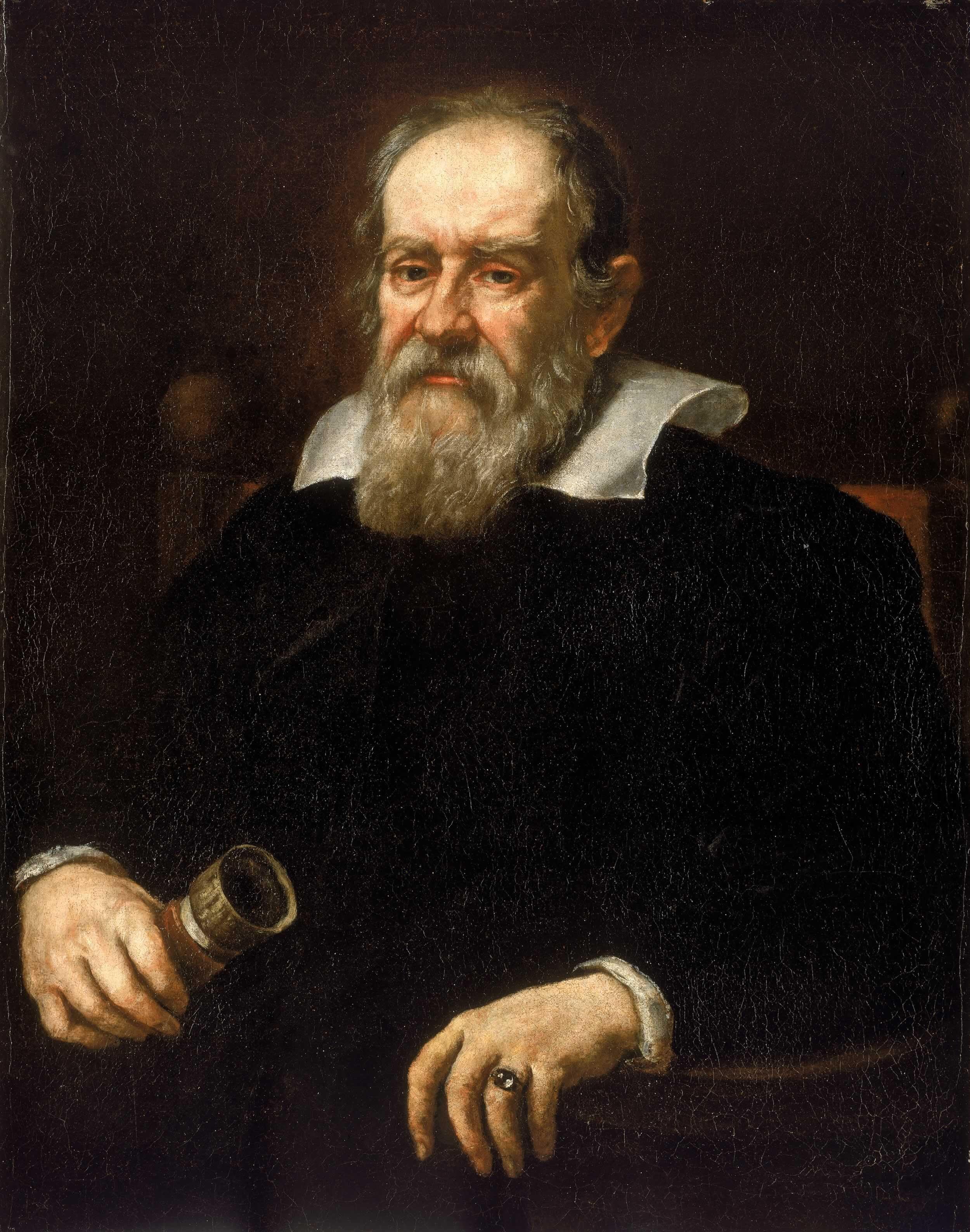
[Original image source](https://www.talmudology.com/jeremybrownmdgmailcom/2021/2/15/happy-birthday-galileo)
**Galileo Galilei(1564—1642)**
Galileo studied not only motion, astronomy, and physics, but also mathematical questions arising from dice games.
In a manuscript usually dated between 1613 and 1623, he discussed a seemingly contradictory phenomenon involving the sum of three dice.
The historical question was:
When three six-sided dice are thrown together, why is a sum of 10 more likely than a sum of 9?
At first, this hardly seems to be a question at all.
We can easily find six different combinations of three dice that sum to 9:
\[
\begin{aligned}
9={}&1+2+6\\
={}&1+3+5\\
={}&1+4+4\\
={}&2+2+5\\
={}&2+3+4\\
={}&3+3+3.
\end{aligned}
\]
For 10, there are also exactly six:
\[
\begin{aligned}
10={}&1+3+6\\
={}&1+4+5\\
={}&2+2+6\\
={}&2+3+5\\
={}&2+4+4\\
={}&3+3+4.
\end{aligned}
\]
If each sum has six combinations, why should their frequencies differ?
Galileo's crucial insight was: **we were counting the wrong objects.**
For example, the combination
\[
1+2+6=9
\]
can actually arise from six ordered outcomes:
\[
(1,2,6),(1,6,2),(2,1,6),
\]
\[
(2,6,1),(6,1,2),(6,2,1).
\]
But
\[
3+3+3=9
\]
has only one permutation.
Although both count as “one combination of face values,” they contain completely different numbers of actual dice outcomes.
Let us carry out the full calculation.
Three dice: all combinations with sums of 9 and 10
**Sum = 9**
| Combination | Permutations |
|---|---:|
| 1,2,6 | 6 |
| 1,3,5 | 6 |
| 1,4,4 | 3 |
| 2,2,5 | 3 |
| 2,3,4 | 6 |
| 3,3,3 | 1 |
| **Total** | **25** |
**Sum = 10**
| Combination | Permutations |
|---|---:|
| 1,3,6 | 6 |
| 1,4,5 | 6 |
| 2,2,6 | 3 |
| 2,3,5 | 6 |
| 2,4,4 | 3 |
| 3,3,4 | 3 |
| **Total** | **27** |
Probability of a sum of 9
25/216
Approximately 11.57%
Probability of a sum of 10
27/216
12.50%
Under a model of three fair, mutually independent dice, we obtain
\[
\boxed{
P(S=10)-P(S=9)=\frac{2}{216}=\frac1{108}.
}
\]
This agrees with the phenomenon Galileo explained. For the manuscript's dating, the problem's background, and the calculation, see Hald's history of probability and the English translation of Galileo's text. 〔[5](#ref-turn689420search25), [6](#ref-turn689420search2), [7](#ref-turn689420search26)〕
What really matters here, however, is not yet the numbers \(25\) and \(27\).
We must instead answer:
**Why can ordered triples be counted with equal weights, while unordered combinations of three face values cannot?**
We cannot merely say that ordered triples give the correct answer.
That would use the answer to justify the method after the fact.
We need a mathematical principle independent of the answer to this particular problem.
That principle is symmetry.
## 1.8 Symmetry: Why Should Certain Outcomes Have the Same Probability?
Imagine an ideal, perfectly symmetric six-sided die.
Its six faces are labeled \(1,2,\ldots,6\).
If its material is distributed uniformly, its shape is perfectly symmetric, and the throwing mechanism favors no face, we have reason to believe that no difference among the faces affects their chances.
Notice that we did not begin by saying
\[
P(1)=\cdots=P(6)=\frac16.
\]
Our starting claim was:
**If two outcomes can be exchanged by a symmetry transformation that leaves the random mechanism unchanged, those outcomes should have the same probability.**
A very general mathematical idea now comes into play:
> The symmetries of an object should constrain the mathematical quantities that describe it.
Let us try to express this rigorously.
Let
\[
\Omega=\{\omega_1,\ldots,\omega_n\}
\]
be a finite outcome space.
Consider transformations acting on \(\Omega\) that form a group \(G\).
Assume:
1. The action of \(G\) on \(\Omega\) is transitive: any two outcomes can be transformed into one another by some group element;
2. The probability assignment under study is invariant under these transformations;
3. The total probability of all outcomes is 1, and the probabilities of mutually exclusive outcomes can be added.
In mathematical language, the second condition is
\[
P(gA)=P(A),
\qquad g\in G,\quad A\subseteq\Omega.
\]
By transitivity, for any \(\omega_i,\omega_j\), there is a \(g\in G\) such that
\[
g\omega_i=\omega_j.
\]
Therefore
\[
P(\{\omega_i\})
=
P(\{\omega_j\}).
\]
All singleton events thus have a common probability \(p\).
By normalization and additivity,
\[
1=P(\Omega)
=\sum_{i=1}^{n}P(\{\omega_i\})
=np.
\]
Hence
\[
\boxed{p=\frac1n}.
\]
For any event \(A\subseteq\Omega\), finite additivity gives
\[
\begin{aligned}
P(A)
&=\sum_{\omega\in A}P(\{\omega\})\\
&=\sum_{\omega\in A}\frac1n\\
&=\frac{|A|}{n}.
\end{aligned}
\]
We finally obtain the very familiar formula:
\[
\boxed{
P(A)=\frac{|A|}{|\Omega|}.
}
\]
But it now has a completely different meaning.
It is no longer a calculation rule that we have simply declared.
**On a finite space, it follows jointly from symmetry, normalization, and additivity.**
There is also a logical distinction that must be emphasized:
We have proved that if a probability assignment satisfies the relevant symmetry, it must be uniform.
We have not proved that real dice necessarily have this probabilistic symmetry.
Mathematics reveals the necessary consequences of symmetry. A symbolic model alone cannot guarantee that reality satisfies the model's assumptions.
### 1.8.1 A Deeper Question: Is Symmetry Objective, or Do We Choose It?
If someone alters a die's center of mass, it still has six labels, but we can no longer assume that its six outcomes are equally likely.
Symmetry therefore does not follow directly from the fact that “there are six outcomes.”
It comes from our judgment about the mechanism that generates the outcomes.
There is, however, another, subtler possibility.
Suppose I know nothing about a die's construction and have never observed any of its throws.
Can I assign equal probabilities to its six faces simply because I lack information?
This concerns what later came to be called the *Principle of Indifference*.
This idea has an important place in classical interpretations of probability, but it has also long been challenged: does not knowing how outcomes differ mean that they do not actually differ? 〔[8](#ref-turn561005search0), [9](#ref-turn561005search3)〕
There are two distinct propositions here:
\[
\text{the mechanism is symmetric}
\]
and
\[
\text{we do not know of any asymmetry in the mechanism}.
\]
The first is a statement about the world.
The second is a statement about our knowledge.
They are not equivalent.
This becomes an enduring disagreement in the history of probability: **does probability describe the objective world, or our uncertain knowledge of it?**
Before settling this philosophical question, however, we face a more immediate mathematical difficulty.
---
## 1.9 Why Does a Correct Probability Calculation Depend on How We Describe Outcomes?
Return to Galileo's three dice.
We originally represented the experimental outcomes as
\[
\Omega=\{1,\ldots,6\}^3.
\]
This is a finite space with
\[
|\Omega|=6^3=216
\]
elements.
Under the model of independent fair dice, each ordered triple has probability
\[
\frac1{216}.
\]
But adding the three face values gives only an integer.
Define the function
\[
S:\Omega\longrightarrow\{3,4,\ldots,18\}
\]
where
\[
S(i,j,k)=i+j+k.
\]
The event we actually care about is
\[
\{S=10\}.
\]
In other words, we are observing not the complete outcome of the three dice, but the information produced by applying a function to it.
Thus
\[
\{S=10\}
=
S^{-1}(\{10\}).
\]
Here \(S^{-1}\) denotes a preimage, not an inverse function.
Therefore
\[
P(S=10)
=
P(S^{-1}(\{10\}))
=
\frac{|S^{-1}(\{10\})|}{216}.
\]
This is why we must count 27 ordered triples rather than just six unordered combinations.
Two levels of description of the same random experiment
Schematic: a mapping merges outcomes, but need not preserve uniformity. The blocks are conceptual illustrations and do not represent the actual numbers of outcomes in the events.
We have uncovered an extremely important mathematical principle:
**A random object having a uniform distribution does not imply that a function of it also has a uniform distribution.**
In modern mathematical language, we have constructed a new probability distribution:
\[
P_S(B)=P(S^{-1}(B)).
\]
Here \(P_S\) is the pushforward measure of the original probability distribution under the map \(S\).
This formula deserves a pause.
On a finite space, it merely says “count how many dice outcomes correspond to each sum.”
Its structure, however, no longer depends on counting itself.
More generally, let
\[
X:(\Omega,\mathcal F,P)\longrightarrow(E,\mathcal E)
\]
be a measurable mapping.
Then the distribution of \(X\) is defined by
\[
\boxed{
P_X(B)=P(X^{-1}(B)),
\qquad B\in\mathcal E.
}
\]
This is the basic construction of the distribution of a random variable in modern probability theory.
We could follow it further, from discrete distributions to continuous distributions, stochastic processes, and random geometric objects.
But we do not need those theories yet.
We need only recognize one fact:
**Probability does more than assign a weight to a number: a mapping transfers the weights originally attached to the outcomes of a random experiment to the object we observe.**
Viewed through modern mathematics, Galileo's three-dice calculation already contains a finite instance of this idea.
---
## 1.10 Back to the Game: We Had Quietly Used Independence Too
Return now to our original game.
A has won three rounds and B has won two. A needs one more win, while B needs two.
To analyze the match, we can imagine the potential results of the next two rounds in advance, even though the actual match may end after the first.
There are four ordered potential outcomes:
\[
AA,\quad AB,\quad BA,\quad BB.
\]
If A wins at least one of the first two rounds, A receives the entire prize.
Thus A's eventual victory corresponds to
\[
\{AA,AB,BA\},
\]
while B's victory corresponds to
\[
\{BB\}.
\]
If each round is fair and the two rounds are independent, then
\[
P(AA)=P(AB)=P(BA)=P(BB)=\frac14.
\]
It follows that
\[
P(\text{A ultimately wins})=\frac34.
\]
This explains why we initially obtained a fair value of 48 gold coins:
\[
64\cdot\frac34=48.
\]
But a deeper question now arises.
If we know only that A and B each have probability \(1/2\) of winning each round, can we conclude that the four outcomes above are equally likely?
We cannot.
### 1.10.1 An Unexpected Counterexample
Let the potential outcomes of the next two rounds be random variables \(X_1,X_2\), taking values in \(\{A,B\}\).
We require only
\[
P(X_1=A)=P(X_1=B)=\frac12
\]
and
\[
P(X_2=A)=P(X_2=B)=\frac12.
\]
That is, each round considered on its own is fair.
This does not mean that the rounds are independent.
In fact, all three models below satisfy these marginal probability conditions.
| Model | \(P(AA)\) | \(P(AB)\) | \(P(BA)\) | \(P(BB)\) |
|---|---:|---:|---:|---:|
| Independent | 1/4 | 1/4 | 1/4 | 1/4 |
| Perfect positive correlation | 1/2 | 0 | 0 | 1/2 |
| Perfect negative correlation | 0 | 1/2 | 1/2 | 0 |
They give exactly the same answer to “Is each round fair?”
Yet they give completely different answers to “Who eventually wins the prize?”
The probability that A eventually wins the prize. Choose independence, perfect positive correlation, or perfect negative correlation, and compare the probabilities of AA, AB, BA, and BB and A's fair share.
This shows that the fairness of each round alone does not determine the eventual winning probability.
We can, in fact, go further.
Let
\[
P(AA)=x.
\]
Since both marginal distributions equal \((1/2,1/2)\), we must have
\[
P(AB)=P(BA)=\frac12-x,
\]
and
\[
P(BB)=x.
\]
where
\[
0\le x\le\frac12.
\]
Thus A's eventual winning probability is
\[
\begin{aligned}
P(\text{A wins})
&=1-P(BB)\\
&=1-x.
\end{aligned}
\]
Without assuming independence, therefore,
\[
\boxed{
\frac12\le P(\text{A wins})\le1.
}
\]
The \(3/4\) we originally calculated is only one particular value in this entire range of possibilities.
Only with the independence assumption,
\[
P(AA)
=
P(X_1=A)P(X_2=A)
=
\frac14,
\]
can we conclude
\[
P(\text{A wins})=\frac34.
\]
For the first time, we have discovered that:
**Knowing the law of each random outcome separately does not mean knowing their joint law.**
This is one way in which probability theory goes deeper than counting alone.
It studies not only how likely an outcome is, but also the relationships among different outcomes.
More importantly, the original recurrence \(V(a,b)\), which expressed value using only the current score, also implicitly assumed that the score contained all relevant information needed to determine the future distribution.
If future outcomes are dependent, and that dependence also depends on the particular past outcomes, the current score alone may be insufficient to calculate future value correctly.
We are already approaching the heart of the later Markov property and the concept of a “state.”
---
## 1.11 Why Should the Probabilities of Mutually Exclusive Events Add?
We have introduced three important ideas:
symmetry, independence, and additivity.
Symmetry tells us when different outcomes should have the same probability.
Independence tells us when a joint probability can be factored into a product of individual probabilities.
But additivity seems to leave a question unanswered:
Why should the probabilities of two mutually exclusive events add?
For example, if \(A\cap B=\varnothing\), why require
\[
P(A\cup B)=P(A)+P(B)?
\]
Is this another rule introduced out of nowhere?
Let us return once more to gambling.
Suppose someone can buy a contract:
it pays one gold coin if event \(A\) occurs, and nothing otherwise.
We write
\[
\mathbf 1_A
\]
for the contract's payoff.
Now consider two contracts:
the first pays one gold coin if event \(A\) occurs.
The second pays one gold coin if event \(B\) occurs.
Assume \(A\) and \(B\) are mutually exclusive.
The total payoff from holding both contracts is
\[
\mathbf1_A+\mathbf1_B.
\]
But since \(A\cap B=\varnothing\),
\[
\boxed{
\mathbf1_A+\mathbf1_B=\mathbf1_{A\cup B}.
}
\]
Notice that this is, first of all, an entirely deterministic algebraic identity.
No probability calculation is involved.
It simply says that when two events cannot happen together, receiving one coin if either event occurs produces exactly the same payoff as separately holding the two corresponding contracts.
Now introduce an idealized principle of pricing without arbitrage:
if two portfolios produce identical payoffs in every possible situation, they should have the same price.
Let
\[
\pi(X)
\]
denote the price of payoff \(X\).
If these contracts can all be freely bought and sold, and the price system must rule out arbitrage opportunities in finite portfolios, consistent pricing must satisfy linear relationships.
In particular,
\[
\pi(\mathbf1_A+\mathbf1_B)
=
\pi(\mathbf1_A)+\pi(\mathbf1_B).
\]
We can therefore define
\[
P(A)=\pi(\mathbf1_A),
\]
normalizing the price of a contract guaranteed to pay one gold coin to 1.
We obtain
\[
\boxed{
P(A\cup B)=P(A)+P(B)
}
\]
whenever \(A\cap B=\varnothing\).
We also obtain
\[
P(\Omega)=1,
\qquad
P(A)\ge0,
\]
where nonnegativity follows from the no-arbitrage requirement that a nonnegative payoff cannot have a negative price.
Thus, in this idealized finite trading model, consistent prices for event contracts yield a finitely additive probability assignment.
This does not mean that probability theory historically arose entirely from financial pricing, or that actual market prices necessarily equal true probabilities.
We have simply discovered, from a modern mathematical perspective, a surprising unity:
**The additivity of probability can be connected to consistent pricing across different bets.**
In this sense, probability can both describe chance and provide a mathematical tool for valuing uncertain payoffs.
This also helps us understand the starting point of Chapter 1 anew.
We originally wanted only to divide 64 gold coins fairly.
Yet to understand “fairly,” we gradually introduced states, symmetry, independence, events, and additivity.
A mathematical structure is emerging from a concrete problem.
---
## 1.12 Counting Eventually Fails
We can now calculate probabilities on finite sample spaces with equally likely outcomes.
But can every probability problem be reduced to some kind of counting?
Suppose someone chooses a real number at random from the interval \([0,1]\).
Consider the interval
\[
\left[0,\frac12\right]
\]
What is the probability that the chosen number lies in it?
Following our earlier formula, we seem to need
\[
\frac{
|\{x:0\le x\le1/2\}|
}{
|\{x:0\le x\le1\}|
}.
\]
But the two intervals have the same cardinality.
Indeed, the mapping
\[
f:[0,1]\longrightarrow\left[0,\frac12\right],
\qquad f(x)=\frac x2
\]
is a bijection.
Thus
\[
\left|\left[0,\frac12\right]\right|
=
|[0,1]|.
\]
Comparing only the numbers of elements in these sets cannot distinguish the intervals at all.
Yet our intuitive understanding of “choosing uniformly from \([0,1]\)” calls for
\[
P\left(X\in\left[0,\frac12\right]\right)=\frac12.
\]
This reveals a fundamental difficulty:
**On infinite sets, the number of elements can no longer play the role of probability directly.**
More precisely, cardinality cannot capture the relative size expressed by interval length.
We need a concept more general than counting:
a tool that assigns a mathematical “size” to sets while retaining the necessary additive properties.
This is one of the problems that measure theory would eventually solve.
We are not ready to construct Lebesgue measure here, because many foundational questions remain to be explored.
But the direction of the story is becoming clear.
Starting from finitely many equally likely outcomes, probability theory must eventually reach a language independent of counting.
Along the way, we will discover a profound fact in the opposite direction:
\[
\text{counting}
\subset
\text{measure}.
\]
Uniform probability on a finite set is merely a special case of a more general measure structure.
---
## What Have We Discovered in This Chapter?
Looking back, we began simply by asking how to divide the prize in an interrupted game.
To obtain a mathematically meaningful answer, however, we discovered:
\[
\boxed{
\text{fair division}
\longrightarrow
\text{future outcomes}
\longrightarrow
\text{symmetry}
\longrightarrow
\text{probability assignment}
}
\]
Studying combinations of outcomes then forced us to introduce independence, additivity, and random mappings.
Most intriguingly, the classical probability formula, which initially seemed so natural,
\[
P(A)=\frac{|A|}{|\Omega|}
\]
does not actually tell us what probability is.
It tells us only how to calculate probability in a particular finite model with an equal-weight structure.
As Laplace's later classical formulation illustrates, the classical approach depends on the crucial premise of “equally possible cases.” What makes those cases equally possible itself still requires explanation. 〔[8](#ref-turn561005search0), [10](#ref-turn561005search25)〕
We have gained some mathematical tools, yet the most fundamental question remains:
**What should we do when outcomes lack symmetry, or when we do not know their probabilities at all?**
This leads us naturally to the next chapter.
# Chapter 2: From Chance to Belief—When Outcomes Are No Longer Equally Likely
In the next chapter, we will begin with an unfair die.
This time we cannot count directly or assume a uniform distribution in advance.
We will ask whether observing random phenomena can gradually reveal their underlying probabilities. If so, how can finite experience support predictions about the future?
There we will encounter two important and distinct directions in early probability theory: studying stable frequencies through repeated trials, and using available information to infer unknown outcomes.
These explorations will eventually lead us to Bernoulli's law of large numbers and the ideas of probabilistic inference advanced by Bayes and Laplace.
The Mathematics of Chance · Volume I, Chapter 1, draft v0.2 · End of chapter
---
# The Mathematics of Chance
Volume I · Can Chance Be Calculated?
# Chapter 2: From Chance to Knowledge—How Do We Discover Unknown Probabilities?
From Jacob Bernoulli's law of large numbers to Thomas Bayes's inverse inference.
In Chapter 1, we discovered something surprising.
An unfinished game of chance forced us to consider fairness, chance, and why a future that has not yet occurred can become an object of mathematical study.
Yet the theory we developed always depended on a special condition:
**We knew the chances of the different outcomes in advance.**
For a fair die, we assumed that all six faces were equally likely. For a fair coin, we assumed that heads and tails had the same probability.
What happens if we no longer know those probabilities?
This time, we cannot move directly from a mathematical model to its outcomes.
We must start from outcomes already observed and work backward to understand the unknown law that generated them.
This will bring a fundamental change to probability theory.
---
## 2.1 An Unfair Coin
Imagine that someone hands us a coin.
We do not know whether it is fair or whether someone has altered it.
We know only that each toss produces heads or tails.
Let the probability of heads be
\[
p.
\]
Unlike in Chapter 1, however, we do not know the value of \(p\).
All we can be sure of is
\[
0\le p\le1.
\]
The question now is:
**Can observing the coin's actual behavior tell us the value of \(p\)?**
Suppose we toss it ten times and obtain seven heads and three tails.
A very natural answer is:
\[
p\approx\frac7{10}=0.7.
\]
But what mathematical basis does this answer have?
If the true value is \(p=1/2\), seven heads in ten tosses is entirely possible.
If the true value is \(p=0.8\), seven heads is also entirely possible.
Even when \(p=0.3\), seven heads is still an event with nonzero probability.
Thus:
\[
\text{observing seven heads}
\not\implies p=0.7.
\]
At most, we can say that some values of \(p\) seem to fit the observation better than others.
But what does “fit better” mean?
Before answering, we need to recognize a more fundamental distinction.
## 2.2 Two Very Different Kinds of Uncertainty
We have encountered two questions pointing in opposite directions.
**First question: given the probability, predict the outcomes.**
If we know that the probability of heads is \(p\), we want to calculate the probability of seven heads in the next ten tosses.
This is a forward probability problem.
**Second question: given the outcomes, infer the probability.**
If we have observed seven heads in ten tosses, we want to infer the unknown \(p\).
This is a problem of inverse inference.
In modern notation, let
\[
X_i=
\begin{cases}
1,&\text{trial }i\text{ is heads},\\
0,&\text{trial }i\text{ is tails}.
\end{cases}
\]
For a given \(p\), assume
\[
X_1,\ldots,X_n
\overset{\mathrm{i.i.d.}}{\sim}\operatorname{Bernoulli}(p).
\]
Define
\[
S_n=\sum_{i=1}^n X_i.
\]
The forward problem studies
\[
P_p(S_n=k).
\]
The inverse problem asks:
after observing \(S_n=k\), what can we conclude about \(p\)?
Although they seem merely to exchange the known and the unknown, the two questions differ substantially in mathematical terms.
In the first, the probability model has already been specified.
In the second, we are trying to understand the probability model itself.
Forward problem
\[
p\text{ known}
\]
\[
P_p(S_n=k)
\]
From law to observation
Inverse problem
\[
S_n=k\text{ known}
\]
\[
p\text{ unknown}
\]
From observation to law
Historically, the move from the mathematics of gambling to inference about the real world was a major turning point in the development of probability.
In dice games, rules and symmetry can give us probabilities.
For human lifespans, disease rates, natural phenomena, or social events, however, we often have no reason to assume equal likelihood in advance.
All we have is what happened in the past.
**If probability theory could handle only problems with known probabilities, it could never become a mathematics of the empirical world.**
Jacob Bernoulli recognized precisely this important direction.
---
## 2.3 Jacob Bernoulli: Can Experience Reveal Probability?
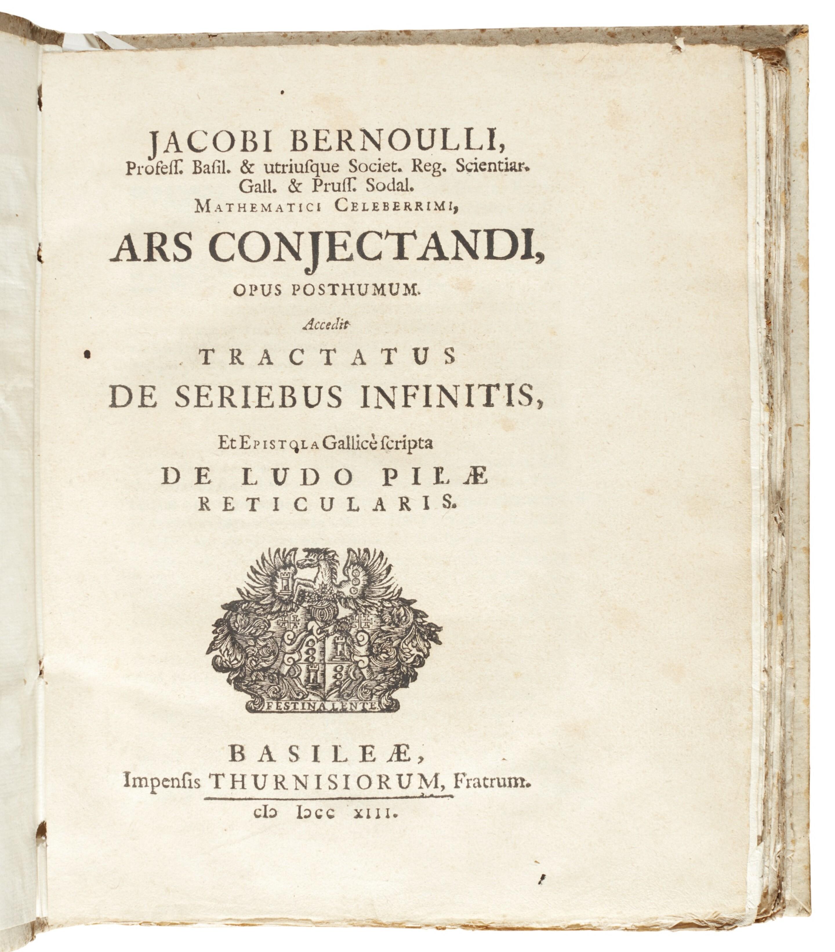
[Original image source](https://www.sothebys.com/en/auctions/ecatalogue/2018/the-library-of-erwin-tomash-l18409/lot.58.html)
**Jacob Bernoulli(1655—1705)**
A Swiss mathematician and an important member of the Bernoulli family, he spent many years studying how to extend the mathematics of games of chance to uncertain problems in everyday life.
His book *Ars Conjectandi* (*The Art of Conjecturing*) was published posthumously in 1713.
The book matters for more than its inclusion of what later became known as the law of large numbers.
Still more significant is the question Bernoulli was trying to answer.
In his day, mathematicians could calculate chances in idealized games because the rules were usually known.
The real world, however, does not tell us its probabilities in advance.
For example:
How likely is a particular disease to be fatal?
What proportion of a population has a certain characteristic?
How frequently will a natural phenomenon occur under specified conditions?
Can repeated observation gradually reveal these unknown proportions?
In *Ars Conjectandi*, Bernoulli sought to extend the mathematics of gambling to civil, moral, and economic matters. His law of large numbers provided a mathematical basis for inferring unknown chances from repeated observations. Historians Edith Dudley Sylla and Ian Hacking have both emphasized the significance of this move from gambling to empirical inference. 〔[11](#ref-turn557906search0), [12](#ref-turn557906search5), [13](#ref-turn557906search11)〕
But an apparent paradox arises.
If we do not know \(p\) to begin with, how can we prove that observed frequencies will get closer and closer to \(p\)?
We seem to need to know the probability before we can justify discovering it through observation.
This was the central mathematical problem Bernoulli faced.
### 2.3.1 Begin with an Urn Whose Proportions Are Known
Consider an urn containing \(r\) red balls and \(s\) black balls.
Each time, draw a ball at random, record its color, put it back, and mix the contents again.
Assume that every ball has the same chance of being drawn.
The probability of drawing red is then
\[
p=\frac{r}{r+s}.
\]
Make \(n\) independent repeated draws.
Define
\[
X_i=\mathbf1_{\{\text{trial }i\text{ draws a red ball}\}}.
\]
The number of red balls drawn is
\[
S_n=X_1+\cdots+X_n.
\]
so the empirical frequency is
\[
\widehat p_n=\frac{S_n}{n}.
\]
We are not asking whether, for some particular finite \(n\), it equals \(p\) exactly.
Even when \(p=1/2\), ten red draws in a row are entirely possible.
The real question is:
for any given accuracy \(\varepsilon>0\), as the number of trials increases, does
\[
|\widehat p_n-p|<\varepsilon
\]
hold with increasingly high probability?
In modern mathematical language, we want to prove:
\[
\boxed{
P_p\left(
\left|\frac{S_n}{n}-p\right|>\varepsilon
\right)\longrightarrow0.
}
\]
This is the modern form of Bernoulli's law of large numbers.
More precisely, it expresses convergence in probability:
\[
\boxed{
\widehat p_n\xrightarrow{P_p}p.
}
\]
Bernoulli proved an early rigorous form of this idea. He studied not only the limit, but also how to make the probability of a deviation smaller than a prescribed number. His argument used the binomial distribution and combinatorics rather than the modern variance inequality we will use next. 〔[14](#ref-turn557906search1), [13](#ref-turn557906search11)〕
## 2.4 Why Can Random Error Disappear?
Let us leave history for a moment and prove this phenomenon anew using modern mathematics.
There is something here well worth considering.
Every toss is random.
Even after a million trials, the million-and-first outcome may still be heads or tails.
If randomness in individual outcomes does not disappear, why can their average become increasingly stable?
The answer lies in the different properties of expectation and variance.
### Step One: From the Total Count to the Average
Since
\[
X_i\sim\operatorname{Bernoulli}(p),
\]
we have
\[
\mathbb E_p[X_i]
=
1\cdot p+0\cdot(1-p)
=p.
\]
Therefore
\[
\mathbb E_p[\widehat p_n]
=
\mathbb E_p\left[\frac1n\sum_{i=1}^nX_i\right]
=p.
\]
The expectation of the empirical frequency always equals the true probability.
But this alone does not allow us to claim that the empirical frequency will be close to the true probability.
For when \(n=1\),
\[
\widehat p_1\in\{0,1\},
\]
its expectation is still \(p\), yet its value may be far from \(p\).
**Expectation tells us a random quantity's average location, but cannot by itself tell us how strongly it fluctuates around that location.**
We are therefore forced to study the fluctuations themselves.
### Step Two: Measure Fluctuations with Variance
For a Bernoulli random variable,
\[
X_i^2=X_i.
\]
Thus
\[
\begin{aligned}
\operatorname{Var}_p(X_i)
&=\mathbb E_p[X_i^2]-(\mathbb E_p[X_i])^2\\
&=p-p^2\\
&=p(1-p).
\end{aligned}
\]
Next consider the variance of the average.
In general,
\[
\operatorname{Var}\left(\sum_{i=1}^nX_i\right)
=
\sum_{i=1}^n\operatorname{Var}(X_i)
+
2\sum_{i
An important mathematical phenomenon appears here:
to halve the standard deviation, we generally need to quadruple the sample size.
This is because
\[
\operatorname{SD}(\widehat p_n)\propto\frac1{\sqrt n}.
\]
This provides the simplest example of the \(\sqrt n\) scale that will appear so often in statistical inference.
Of course, we have studied only second moments so far; we have not proved a more detailed limiting distribution.
### Step Three: From Mean Squared Error to a Probability Statement
We already know
\[
\mathbb E_p[(\widehat p_n-p)^2]
=
\frac{p(1-p)}n.
\]
But the law of large numbers requires control of
\[
P_p(|\widehat p_n-p|\ge\varepsilon).
\]
How can we turn a statement about expectation into a statement about probability?
Notice that for every real number \(y\),
\[
\mathbf1_{\{|y|\ge\varepsilon\}}
\le\frac{y^2}{\varepsilon^2}.
\]
Therefore
\[
\begin{aligned}
P_p(|\widehat p_n-p|\ge\varepsilon)
&=\mathbb E_p\left[
\mathbf1_{\{|\widehat p_n-p|\ge\varepsilon\}}
\right]\\
&\le
\frac{\mathbb E_p[(\widehat p_n-p)^2]}
{\varepsilon^2}\\
&=\frac{p(1-p)}{n\varepsilon^2}.
\end{aligned}
\]
Since
\[
p(1-p)\le\frac14,
\]
we obtain
\[
\boxed{
P_p(|\widehat p_n-p|\ge\varepsilon)
\le\frac1{4n\varepsilon^2}.
}
\]
For each fixed \(\varepsilon>0\), the right-hand side tends to zero.
Thus
\[
\boxed{\widehat p_n\xrightarrow{P_p}p.}
\]
This completes the proof.
The proof is short, but it reveals a deep structure.
We have not made individual random events deterministic.
We have proved only that averaging sufficiently many independent random events constrains the fluctuations of their average more and more tightly.
**Randomness has not disappeared; what disappears is the chance that the average deviates from its center.**
### 2.4.1 Where Exactly Does Independence Enter?
Look at the proof again.
The expectation step,
\[
\mathbb E\left[\frac1n\sum X_i\right]
=
\frac1n\sum\mathbb E[X_i]
\]
does not require independence.
Independence is actually used in
\[
\operatorname{Var}\left(\sum X_i\right)
=
\sum\operatorname{Var}(X_i).
\]
If the random variables are correlated, their covariances may not be negligible.
For example, suppose
\[
X_1=X_2=\cdots=Y
\]
and \(Y\sim\operatorname{Bernoulli}(p)\).
All trial outcomes are then identical.
Although each \(X_i\) still has marginal distribution Bernoulli\((p)\),
\[
\widehat p_n=Y
\]
for every \(n\).
Increasing the number of repetitions therefore produces no stabilization at all.
The law of large numbers thus depends on more than the surface fact that “we performed many trials.”
More fundamentally, **the dependence among trials must be weak enough to control the average error.**
Independence is a particularly effective sufficient condition, but it is not the only possible hypothesis for a law of large numbers.
We will return to this question repeatedly when studying ergodic theory, martingales, and dependent stochastic processes.
---
## 2.5 What Does the Law of Large Numbers Answer, and What Does It Leave Open?
We have now proved an important conclusion:
\[
\widehat p_n\xrightarrow{P_p}p.
\]
At first sight, this seems to solve the problem of inferring an unknown probability.
If we observe enough trials, the empirical frequency will approach the true probability.
But a logical difficulty is hidden here.
The law of large numbers says:
> Assuming the true probability is \(p\), the empirical frequency is likely to be close to \(p\).
What we want to conclude is:
> I have observed an empirical frequency of \(0.7\), so the true probability should be close to \(0.7\).
These statements look similar, but they are not the same logical proposition.
One predicts observations from a model.
The other infers a model from observations.
We cannot simply reverse the direction of a conditional probability statement without proof.
### 2.5.1 How Can the Law of Large Numbers Become an Actual Method of Inference?
Fortunately, its probability inequality provides a more rigorous approach.
We proved earlier that
\[
P_p(|\widehat p_n-p|\ge\varepsilon)
\le\frac1{4n\varepsilon^2}.
\]
Notice that the inequality holds for every \(p\in[0,1]\).
Even without knowing \(p\), we can therefore prescribe an acceptable error probability \(\delta\in(0,1)\) in advance.
Set
\[
\varepsilon_n=\sqrt{\frac1{4n\delta}}.
\]
Then
\[
P_p\left(
|\widehat p_n-p|\le\varepsilon_n
\right)\ge1-\delta.
\]
Now define a random interval determined by the observed data:
\[
\boxed{
C_n=
\left[
\widehat p_n-\varepsilon_n,
\widehat p_n+\varepsilon_n
\right]\cap[0,1].
}
\]
For every true parameter \(p\), we then have
\[
\boxed{
P_p(p\in C_n)\ge1-\delta.
}
\]
This is a parameter-inference procedure with a rigorous coverage guarantee.
For example, suppose we make 100 independent tosses and observe 70 heads.
Take \(\delta=0.05\).
Then
\[
\varepsilon_{100}
=
\sqrt{\frac1{4(100)(0.05)}}
\approx0.224.
\]
giving the interval
\[
C_{100}\approx[0.476,0.924].
\]
This interval is indeed very wide.
Its advantage, however, is a coverage guarantee of at least 95%, obtained without any prior guess about the unknown \(p\).
Modern statistics can improve this substantially through sharper inequalities or exact binomial methods. This construction is intended only to make the mathematical principle clear.
### 2.5.2 A Subtle Philosophical Question
Now suppose we have indeed observed 70 heads and calculated this fixed interval.
Can we say:
“The probability that the true parameter lies in this interval is at least 95%”?
That interpretation does not follow directly within the mathematical framework just used.
The reason is that \(p\) is treated as a fixed but unknown parameter.
Before the experiment, the interval \(C_n\) is random. It may or may not contain the true parameter.
Once we observe particular data, however, the interval is determined.
Coverage means: **if we repeatedly use this construction in repeated experiments with the same true parameter, at least 95% of the intervals will contain it.**
It does not directly assign a 95% conditional probability to the already fixed parameter.
Yet from the practical human position of facing an unknown, another question is almost inevitable:
since we do not know \(p\), why can we not assign a probability to \(p\) itself?
For example:
\[
P(0.60.
}
\]
The correlations among tosses in this model are therefore generated by their common unknown parameter.
This is an extremely important mathematical structure.
We began with simple conditionally independent trials. By mixing distributions associated with different parameters, we produced a random sequence that is dependent overall.
The sequence also has a special property.
For any positive integer \(n\) and any \(x_1,\ldots,x_n\in\{0,1\}\), let
\[
k=\sum_{i=1}^n x_i.
\]
Then
\[
\begin{aligned}
&P(X_1=x_1,\ldots,X_n=x_n)\\
&\qquad =
\int_0^1\theta^k(1-\theta)^{n-k}\,d\theta.
\end{aligned}
\]
The right-hand side depends only on the total number of successes \(k\), not on the particular order of successes and failures.
Thus, for every permutation \(\sigma\),
\[
\boxed{
(X_1,\ldots,X_n)
\overset d=
(X_{\sigma(1)},\ldots,X_{\sigma(n)}).
}
\]
We have obtained an exchangeable random sequence.
This is not independence, but it is a symmetry stronger than merely having identical marginal distributions.
We will return to this when studying de Finetti's theorem.
For infinite Bernoulli sequences, de Finetti's theorem will reveal a striking connection between exchangeability and mixtures of conditionally independent models.
For now, let us keep this discovery in mind.
It reveals a fact that was previously easy to overlook:
> **How we handle unknown structure within a random system can itself determine the dependence among the random variables we observe.**
---
## 2.10 Have We Merely Replaced “Not Knowing” with Another Assumption?
Our story seems complete.
We do not know the coin's true bias.
So we introduce a random parameter \(\Theta\).
After observing data, we calculate its posterior distribution using conditional probability.
Finally, we use the posterior to predict the future.
But what justified our initial assumption
\[
\Theta\sim\operatorname{Uniform}(0,1)
\]
in the first place?
In the earlier physical experiment, we explicitly specified a device that generated the parameter uniformly at random.
That distribution therefore had a basis in the model.
If instead we find a coin in the real world, we do not know how its bias arose.
Choosing a uniform prior then becomes a modeling decision requiring justification.
Even the word “uniform” is less simple than it seems.
Suppose that instead of \(\Theta\), we study
\[
U=\Theta^2.
\]
If \(\Theta\sim\operatorname{Uniform}(0,1)\), then for \(0\le u\le1\),
\[
\begin{aligned}
P(U\le u)
&=P(\Theta^2\le u)\\
&=P(\Theta\le\sqrt u)\\
&=\sqrt u.
\end{aligned}
\]
The density of \(U\) is therefore
\[
\boxed{
f_U(u)=\frac1{2\sqrt u},\qquad 0\varepsilon
\right).
\]
A Bayesian hierarchical model instead first assigns a probability distribution to the unknown parameter, then updates it with data.
Here we study
\[
P(\Theta\in A\mid X_1,\ldots,X_n).
\]
The two approaches treat the “unknown parameter” differently in mathematical terms.
Yet they share an extremely important aim:
**Both seek to learn unknown laws gradually through observation.**
In the beta–Bernoulli model above, we can even see their connection directly.
Since, given \(\Theta=\theta\), the variables \(X_i\) are independent and identically distributed, the corresponding strong law of large numbers gives
\[
P\left(
\left.
\lim_{n\to\infty}\frac{S_n}{n}=\theta
\,\right|\,\Theta=\theta
\right)=1
\]
for prior-almost every \(\theta\).
Integrating over the distribution of \(\Theta\) yields
\[
\boxed{
\frac{S_n}{n}\xrightarrow{\mathrm{a.s.}}\Theta.
}
\]
On the other hand, we have already proved that the posterior mean satisfies
\[
\left|
\mathbb E[\Theta\mid S_n]-\frac{S_n}{n}
\right|
\le\frac1{n+2}.
\]
Therefore
\[
\boxed{
\mathbb E[\Theta\mid S_n]
\xrightarrow{\mathrm{a.s.}}\Theta.
}
\]
In this particular model, as observations accumulate, the posterior mean approaches the random parameter value that actually generated the data.
There is another structure here that was revealed systematically only later.
Since
\[
M_n=
\mathbb E[\Theta\mid X_1,\ldots,X_n],
\]
the tower property of conditional expectation gives
\[
\mathbb E[M_{n+1}\mid X_1,\ldots,X_n]=M_n.
\]
Thus \((M_n)\) is a bounded martingale.
This is a connection worth remembering.
We began by asking only how to predict the next toss.
Yet in modern probability theory, that very prediction process naturally becomes a martingale.
When we later study conditional expectation and stochastic processes, we will be able to reinterpret this chapter's calculations about learning and accumulating information.
---
# Closing Reflections: From Calculating Chance to Forming Knowledge
In Chapter 1, we asked:
**If the chances are known, how should we calculate outcomes?**
Chapter 2 took a further step:
**If the chances are unknown, can observation reveal them?**
Bernoulli found that independent repeated trials allow empirical frequencies to approach hidden probabilities in a stable way.
Bayes's inverse problem showed further that we can construct a probability model for an unknown probability and update our inferences through observation.
These two directions later developed into rich statistical traditions with long-running disagreements.
But together they reveal something.
Probability theory is more than the mathematics of chance outcomes.
It gradually becomes a mathematics of **how people acquire reliable knowledge in an uncertain world**.
“Reliable” does not mean that every inference must be correct. It means that we can state clearly which assumptions an inference depends on, what probabilistic guarantees it has, and how it might fail.
Yet one difficulty in our story remains unresolved.
We proved:
\[
\frac{S_n}{n}\xrightarrow{P}p.
\]
This says only that the probability of a deviation beyond a fixed accuracy tends to zero.
It does not tell us:
when \(n\) is large but finite, how exactly does the empirical frequency fluctuate around \(p\)?
To predict those fluctuations more precisely, we must study
\[
\sqrt n(\widehat p_n-p).
\]
Why does \(\sqrt n\) appear?
Why do so many apparently different random phenomena show nearly the same distributional shape after appropriate standardization?
This brings us to another major discovery in the history of probability:
**the normal distribution and the central limit theorem.**
Before continuing, however, we must trace an older mathematical question: why do the binomial coefficients
\[
\binom nk
\]
produce an approximately bell-shaped curve in repeated trials? And why can that curve eventually extend beyond dice, coins, and the binomial distribution to become an important tool for describing natural errors?
Next: Chapter 3, “The Birth of the Bell Curve—From the Binomial to the Normal Distribution”
The Mathematics of Chance · Volume I, Chapter 2 · Working draft v0.1
---
# The Mathematics of Chance
Volume I · Can Chance Be Calculated?
# Chapter 3: The Birth of the Bell Curve—Why Do Countless Random Phenomena Approach the Same Distribution?
From Abraham de Moivre's binomial approximation to Laplace's general limit theorem, and then to Gauss's theory of errors.
By the end of Chapter 2, we had learned something surprising:
If \(X_1,X_2,\ldots\) are independent, identically distributed Bernoulli\((p)\) random variables, then
\[
\frac1n\sum_{i=1}^nX_i\xrightarrow{P}p.
\]
In other words, a large number of repeated random experiments exhibits an increasingly stable regularity.
But a closer look reveals that this is only half the story.
The law of large numbers tells us where a random average will eventually go, but does not fully explain how it fluctuates on its way to that limit.
Suppose we know that a coin is fair.
After ten thousand tosses, five thousand heads would clearly be perfectly ordinary.
But what about five thousand one hundred heads?
Five thousand two hundred?
Five thousand five hundred?
Of course, we can calculate the exact probability of each outcome. But if the number of repetitions reaches a million, a billion, or more, calculating the binomial coefficients directly becomes extraordinarily cumbersome.
A new mathematical question therefore arises:
**Can we find a mathematical law that approximately describes the entire shape of the random fluctuations, without calculating every possible outcome separately?**
This question eventually led mathematicians to discover one of the most famous functions in probability theory:
\[
\boxed{
\varphi(x)=\frac1{\sqrt{2\pi}}e^{-x^2/2}.
}
\]
Today we call this the standard normal density.
But we will not simply introduce it as a definition.
We want to understand why calculations involving coins and binomial coefficients led mathematicians to an expression containing the exponential function and the constant pi.
In particular:
**Why should \(\pi\) ultimately appear in a random experiment that has nothing to do with circles?**
---
## 3.1 Bernoulli's Unfinished Question: Knowing That the Error Vanishes Is Not Enough
Suppose
\[
S_n=X_1+\cdots+X_n,
\qquad
X_i\overset{\mathrm{i.i.d.}}{\sim}\operatorname{Bernoulli}(1/2).
\]
We know that
\[
S_n\sim\operatorname{Binomial}(n,1/2).
\]
Thus
\[
P(S_n=k)=\binom nk2^{-n}.
\]
For even \(n\), the most likely outcome is
\[
k=\frac n2.
\]
because
\[
\frac{P(S_n=k+1)}{P(S_n=k)}
=
\frac{n-k}{k+1}.
\]
When \(k\) lies to the left of the center, successive probabilities tend to increase; after passing the center, they begin to decrease.
The shape of the binomial distribution must therefore be as follows:
It rises gradually from the left, reaches its maximum in the middle, and then falls to the right.
But this is only a qualitative description.
We still do not know precisely how fast it rises and falls.
First consider a somewhat counterintuitive fact.
As \(n\) increases, the empirical frequency
\[
\widehat p_n=\frac{S_n}{n}
\]
gets closer and closer to \(1/2\).
Yet the probability of obtaining exactly half heads,
\[
P(S_n=n/2)
\]
does not approach 1.
In fact, we will prove that it approaches 0 instead.
This means that
\[
\boxed{
\text{getting closer to the center}
\ne
\text{becoming more likely to equal the center exactly}.
}
\]
Why?
Because as the number of experiments increases, the relative error shrinks, while the absolute fluctuations in the number of successes grow.
We already know that
\[
\operatorname{Var}(S_n)=\frac n4,
\]
so
\[
\operatorname{SD}(S_n)=\frac{\sqrt n}{2}.
\]
The typical scale of fluctuations in the number of successes is \(\sqrt n\), rather than a fixed constant.
As the number of tosses grows, the probability mass therefore spreads across an increasing number of integers near the center.
The probability of any single integer may shrink, while the total probability of a suitably expanding central region can remain high.
This is precisely the structure we will study next.
---
## 3.2 Abraham de Moivre: How Can We Calculate an Almost Incalculable Binomial Expression?
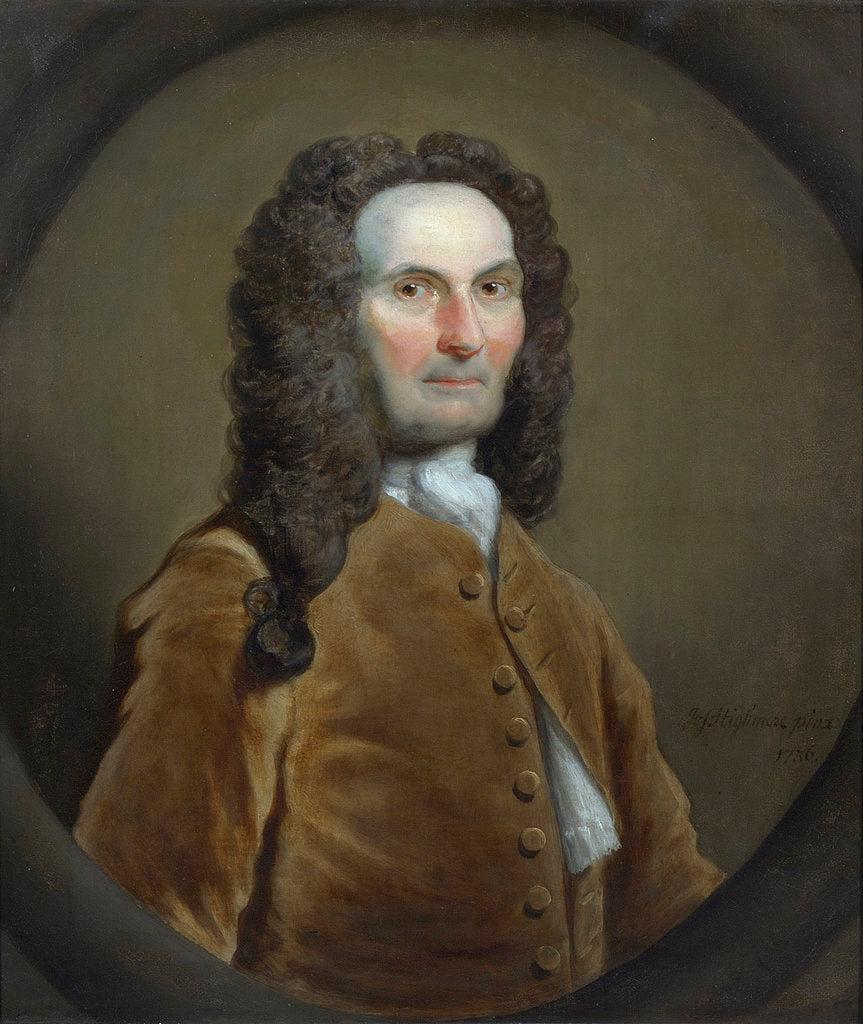
[Original image source](https://prints.royalsociety.org/collections/vintage-mathematics-prints-and-parabola-drawings/products/portrait-of-abraham-de-moivre-1667-1754-rs-9548?utm_source=chatgpt.com)
**Abraham de Moivre(1667—1754)**
A French-born mathematician who later spent much of his life in Britain. In addition to probability, he studied trigonometric analysis and the mathematics of annuities.
In 1733, he wrote the Latin paper *Approximatio ad Summam Terminorum Binomii* on sums of terms in high powers of a binomial. An English version appeared in the second edition of *The Doctrine of Chances* in 1738.
The problem de Moivre faced was very concrete.
In the expansion of a high power of a binomial, we can write every term exactly:
\[
(a+b)^n
=
\sum_{k=0}^n\binom nk a^kb^{n-k}.
\]
But when \(n\) is large, calculating the sum of many neighboring terms becomes very difficult.
And probability problems frequently require exactly this kind of summation.
For example, when \(p=1/2\),
\[
P(a\le S_n\le b)
=
2^{-n}\sum_{k=a}^b\binom nk.
\]
In his 1733 work, de Moivre investigated how a continuous mathematical expression could approximate these sums of binomial coefficients. His main early breakthrough concerned the symmetric binomial distribution; Laplace later extended the underlying ideas considerably. 〔[22](#ref-turn234816search0), [23](#ref-turn234816search4), [24](#ref-turn234816search30)〕
We will now follow his central idea and reconstruct the derivation using modern asymptotic analysis.
### 3.2.1 Begin with the Central Term
To simplify the notation, let
\[
n=2m.
\]
Then
\[
P(S_{2m}=m)
=
\binom{2m}{m}2^{-2m}
=
\frac{(2m)!}{(m!)^2\,4^m}.
\]
Calculating the factorials directly is inconvenient.
But we can use Stirling's formula:
\[
\boxed{
n!\sim\sqrt{2\pi n}\left(\frac ne\right)^n.
}
\]
Here the notation
\[
a_n\sim b_n
\]
means
\[
\lim_{n\to\infty}\frac{a_n}{b_n}=1.
\]
This formula has a history well worth studying in its own right. Both de Moivre and James Stirling made important contributions to factorial asymptotics, and identifying the correct constant \(\sqrt{2\pi}\) was a crucial step. 〔[25](#ref-turn234816search3)〕
Now substitute it into the central binomial coefficient.
\[
(2m)!\sim\sqrt{4\pi m}\left(\frac{2m}{e}\right)^{2m},
\]
\[
(m!)^2\sim 2\pi m\left(\frac me\right)^{2m}.
\]
Therefore
\[
\begin{aligned}
P(S_{2m}=m)
&=\frac{(2m)!}{(m!)^2\,4^m}\\
&\sim
\frac{
\sqrt{4\pi m}(2m/e)^{2m}
}{
2\pi m(m/e)^{2m}4^m
}\\
&=\frac1{\sqrt{\pi m}}.
\end{aligned}
\]
Since \(n=2m\), we can also write
\[
\boxed{
P(S_n=n/2)\sim\sqrt{\frac2{\pi n}}.
}
\]
We have at last reached an important conclusion.
The probability of obtaining exactly half heads is of order
\[
\frac1{\sqrt n}.
\]
Hence
\[
P(S_n=n/2)\longrightarrow0.
\]
This explains the apparently contradictory phenomenon raised at the beginning of the chapter.
But the probability at the center alone does not tell us the shape of the whole distribution.
We must go on to ask:
How large are the terms a certain distance from the center, compared with the central term?
### 3.2.2 Moving Away from the Center
Again let \(n=2m\).
Define
\[
p_m(j)=P(S_{2m}=m+j).
\]
By symmetry,
\[
p_m(j)=p_m(-j).
\]
so we need only consider \(j\ge0\).
The relation between binomial coefficients gives
\[
\frac{p_m(j)}{p_m(0)}
=
\frac{\binom{2m}{m+j}}{\binom{2m}{m}}.
\]
Simplifying yields
\[
\frac{p_m(j)}{p_m(0)}
=
\frac{m!\,m!}{(m+j)!(m-j)!}.
\]
Expanding this further as a product,
\[
\boxed{
\frac{p_m(j)}{p_m(0)}
=
\prod_{r=1}^j\frac{m-r+1}{m+r}.
}
\]
This expression is intriguing.
We have transformed a ratio of enormous binomial coefficients into a product of factors close to 1.
How can we analyze the product of many numbers close to 1?
Taking logarithms is a natural choice.
Logarithms turn products into sums:
\[
\log\frac{p_m(j)}{p_m(0)}
=
\sum_{r=1}^j
\log\left(\frac{m-r+1}{m+r}\right).
\]
Write each term as
\[
\log\left(1-\frac{r-1}{m}\right)
-
\log\left(1+\frac rm\right).
\]
Now use the Taylor expansion
\[
\log(1+x)=x-\frac{x^2}{2}+O(x^3),
\]
valid for \(x\) near 0.
Provided \(j\) does not grow too quickly relative to \(m\), we can control all these expansions.
For \(j=O(\sqrt m)\), the leading terms after summation are
\[
\begin{aligned}
\log\frac{p_m(j)}{p_m(0)}
&=
-\frac1m\sum_{r=1}^j(2r-1)+o(1)\\
&=-\frac{j^2}{m}+o(1).
\end{aligned}
\]
Here we have used
\[
\sum_{r=1}^j(2r-1)=j^2.
\]
Consequently,
\[
\frac{p_m(j)}{p_m(0)}
\sim e^{-j^2/m}.
\]
Combining this with the approximation to the central term,
\[
p_m(0)\sim\frac1{\sqrt{\pi m}},
\]
we finally obtain
\[
\boxed{
P(S_{2m}=m+j)
\sim
\frac1{\sqrt{\pi m}}e^{-j^2/m}
}
\]
where \(j=O(\sqrt m)\). More precisely, the approximation errors can be controlled uniformly over any fixed central window \(|j|\le C\sqrt m\).
Here a completely new functional form suddenly appears:
\[
e^{-j^2/m}.
\]
We did not assume a normal distribution.
We have not even discussed continuous probability densities.
**The squared term in the exponent arises naturally from the structure of binomial coefficients and the Taylor expansion of the logarithm.**
This is the mathematical origin of the bell curve.
## 3.3 Why Must We Standardize by \(\sqrt n\)?
We have just derived
\[
P(S_{2m}=m+j)
\approx
\frac1{\sqrt{\pi m}}e^{-j^2/m}.
\]
An important question now arises.
If we let \(m\to\infty\) while keeping \(j\) fixed, then
\[
\frac{j^2}{m}\to0.
\]
and therefore
\[
e^{-j^2/m}\to1.
\]
This means that, for fixed \(j\), the probabilities at different positions near the center gradually become almost equal.
We would then lose sight of the distribution's actual shape.
We must therefore find the right scale of observation.
Look at the exponent
\[
\frac{j^2}{m}.
\]
If it is to retain nontrivial variation as \(m\to\infty\), we should take
\[
j\asymp\sqrt m.
\]
This is why the square-root scale appears naturally.
It does not come from knowing the definition of standard deviation in advance, or from trying to force a normal distribution to appear.
It comes from the fact that only at this scale do the relative probabilities near the center of the binomial distribution have a nontrivial limiting shape.
Now define
\[
Z_n=\frac{S_n-n/2}{\sqrt n/2}.
\]
This subtracts the expected number of successes and divides by the standard deviation.
When \(n=2m\) and \(S_n=m+j\),
\[
Z_n=\frac{2j}{\sqrt n}.
\]
Let
\[
z=\frac{2j}{\sqrt n}.
\]
Then
\[
\frac{j^2}{m}=\frac{z^2}{2}.
\]
The earlier approximation therefore becomes
\[
P\left(Z_n=z\right)
\approx
\sqrt{\frac2{\pi n}}e^{-z^2/2},
\]
where \(z\) must be a lattice value that \(Z_n\) can actually take.
The distance between adjacent lattice points is
\[
\Delta z=\frac2{\sqrt n}.
\]
Thus
\[
\begin{aligned}
P(Z_n=z)
&\approx
\frac2{\sqrt n}\cdot
\frac1{\sqrt{2\pi}}e^{-z^2/2}\\
&=\Delta z\,\varphi(z).
\end{aligned}
\]
where
\[
\boxed{
\varphi(z)=\frac1{\sqrt{2\pi}}e^{-z^2/2}.
}
\]
Now the picture becomes particularly clear.
The original binomial distribution consists of discrete probability masses.
But as \(n\to\infty\), the spacing between successive standardized values shrinks.
The probability mass at each value is approximately
\[
\text{interval width}\times\text{height of a continuous function}.
\]
We have found that continuous function:
\[
\varphi(z).
\]
This is the mathematical process by which the bell curve emerges from discrete probability.
### 3.3.1 Watching the Bell Curve Emerge
Below, the binomial probability masses for different values of \(n\) are divided by the lattice spacing and compared with the standard normal density.
The lines connecting discrete lattice points in the figure serve only as a visual comparison; they do not mean that the binomial distribution itself has a continuous density.
As \(n\) increases, the correctly standardized discrete probability masses approach the same continuous function.
There is another point worth noticing.
We have not changed the coin itself.
Every toss still has only two outcomes: heads and tails.
**The continuous bell curve is not the shape of an individual random experiment. It is a limiting structure that emerges when many discrete random outcomes are added and rescaled.**
---
## 3.4 From Sums of Binomial Coefficients to Integrals
We now have a local approximation:
\[
P(Z_n=z_{n,k})
\approx
\Delta z_n\,\varphi(z_{n,k}),
\]
where
\[
z_{n,k}=\frac{k-n/2}{\sqrt n/2},
\qquad
\Delta z_n=\frac2{\sqrt n}.
\]
But de Moivre's original goal was not merely to approximate a single binomial coefficient.
He was interested in sums of many terms.
Take any fixed real numbers \(a Editorial supplement: Appendix D controls the remainder in the second-order expansion of the characteristic function; no third-moment assumption is added here.
We already know how to derive the normal distribution from the binomial expansion.
But if \(X_i\) have an entirely different distribution, the binomial-coefficient method no longer applies.
We need a new mathematical language.
This problem will lead us to the deep connection between probability theory and Fourier analysis.
### 3.6.1 Why Study Complex Exponentials?
Suppose the distribution of a random variable \(X\) is very complicated.
Studying the distribution of its independent sum
\[
S_n=X_1+\cdots+X_n
\]
directly usually involves repeated convolution.
For example, if \(X,Y\) are independent with densities \(f_X,f_Y\), then
\[
f_{X+Y}(z)
=
\int_{\mathbb R}f_X(x)f_Y(z-x)\,dx.
\]
For \(n\) random variables, we must convolve repeatedly.
This is a fairly complicated operation.
But mathematicians had already found in other settings that certain functional transforms turn complicated operations into simple algebra.
Define the characteristic function of a random variable \(X\) by
\[
\boxed{
\phi_X(t)=\mathbb E[e^{itX}],
\qquad t\in\mathbb R.
}
\]
The definition may seem rather unexpected.
Why introduce the imaginary unit \(i\)?
Why choose the exponential function in particular?
Because it has a very useful property:
\[
e^{it(x+y)}=e^{itx}e^{ity}.
\]
Thus, if \(X,Y\) are independent,
\[
\begin{aligned}
\phi_{X+Y}(t)
&=\mathbb E[e^{it(X+Y)}]\\
&=\mathbb E[e^{itX}e^{itY}]\\
&=\mathbb E[e^{itX}]\mathbb E[e^{itY}]\\
&=\phi_X(t)\phi_Y(t).
\end{aligned}
\]
and consequently
\[
\boxed{
\phi_{X+Y}(t)=\phi_X(t)\phi_Y(t).
}
\]
We have turned addition of random variables into multiplication of characteristic functions.
The idea resembles our earlier use of logarithms to turn products into sums:
**When faced with a complicated operation, seek a representation in which its difficult structure becomes a simple algebraic relation.**
> Dependencies on later theory: The following is a reconstruction of historical results in modern language, not de Moivre's or Laplace's original proof. Appendix D controls the remainder in the second-order expansion; Chapter 6 develops integration for complex-valued random variables; Chapter 11 systematically prove uniqueness of characteristic functions and Lévy's continuity theorem. Chapter 7 first distinguishes the relevant notions of convergence. This section continues the story through products and second-order terms, without presenting these outside results as if they had been proved here.
### 3.6.2 Proving the Central Limit Theorem Again with Characteristic Functions
Let
\[
Y_i=\frac{X_i-\mu}{\sigma}.
\]
Then
\[
\mathbb E[Y_i]=0,
\qquad
\mathbb E[Y_i^2]=1.
\]
The standardized random sum can be written as
\[
Z_n=\frac1{\sqrt n}\sum_{i=1}^nY_i.
\]
We now examine the characteristic function of \(Y_i\) near \(t=0\).
Using
\[
e^{ity}=1+ity-\frac{t^2y^2}{2}+\cdots,
\]
we expect
\[
\phi_Y(t)
=
1+it\mathbb E[Y]
-\frac{t^2}{2}\mathbb E[Y^2]
+o(t^2).
\]
Since the mean is 0 and the variance is 1,
\[
\boxed{
\phi_Y(t)=1-\frac{t^2}{2}+o(t^2).
}
\]
We do not need to assume that \(Y\) has a third moment.
A finite second moment suffices for this expansion. A rigorous proof can use
\[
\frac{e^{iu}-1-iu}{u^2}\longrightarrow-\frac12
\]
and the corresponding boundedness to control the expectation and obtain the second-order expansion.
Now, because \(Y_1,\ldots,Y_n\) are independent,
\[
\begin{aligned}
\phi_{Z_n}(t)
&=
\prod_{i=1}^n
\phi_{Y_i}\left(\frac{t}{\sqrt n}\right)\\
&=
\left[
\phi_Y\left(\frac{t}{\sqrt n}\right)
\right]^n.
\end{aligned}
\]
Using the Taylor expansion above,
\[
\phi_Y\left(\frac{t}{\sqrt n}\right)
=
1-\frac{t^2}{2n}+o\left(\frac1n\right).
\]
Therefore
\[
\phi_{Z_n}(t)
=
\left[
1-\frac{t^2}{2n}+o\left(\frac1n\right)
\right]^n.
\]
Recall the elementary limit
\[
\left(1+\frac an+o\left(\frac1n\right)\right)^n
\longrightarrow e^a.
\]
It follows that
\[
\boxed{
\lim_{n\to\infty}\phi_{Z_n}(t)
=
e^{-t^2/2}.
}
\]
But
\[
e^{-t^2/2}
\]
is precisely the characteristic function of a standard normal random variable.
The continuity theorem for characteristic functions therefore gives
\[
\boxed{Z_n\xrightarrow d N(0,1).}
\]
This completes the proof.
This modern proof differs from de Moivre's and Laplace's original derivations, but reveals the central mathematical mechanism of the central limit theorem.
### 3.6.3 Why Does Only the Second-Order Term Survive?
Look again at
\[
\phi_Y(t)=1-\frac{t^2}{2}+o(t^2).
\]
When standardizing the sum, we replace \(t\) by \(t/\sqrt n\).
The second-order term becomes
\[
\frac{t^2}{n}.
\]
Multiplying the characteristic functions of \(n\) independent random variables produces a nontrivial limit:
\[
n\cdot\frac{t^2}{n}=t^2.
\]
Under suitable moment conditions, the higher-order terms gradually disappear.
For example, if the third moment exists, the accumulated third-order contribution is of order
\[
n\left(\frac t{\sqrt n}\right)^3
=
\frac{t^3}{\sqrt n}
\to0.
\]
The fourth-order term gives
\[
n\left(\frac t{\sqrt n}\right)^4
=
\frac{t^4}{n}
\to0.
\]
Thus only the second-order structure survives in the limit.
This explains why independent sums from many different distributions have the same limit.
We do not need to know every detail of each distribution.
At this limiting scale, many higher-order details become invisible.
And the characteristic function supplied by the second-order term,
\[
e^{-t^2/2}
\]
corresponds precisely to the normal distribution.
The central limit theorem therefore does much more than happen to announce that sums of many random variables “look bell-shaped.”
It expresses the following mathematical principle:
**Independent summation and square-root standardization preserve second-order structure in the limit while diminishing other local details.**
This is a central reason for the universality of the normal distribution.
---
## 3.7 Gauss: Why Do Astronomers Also Encounter the Bell Curve?
So far, we have discovered the normal distribution by following a path through gambling, binomial expressions, and independent random sums.
Historically, another important path led to the same function.
It began not with dice,
but with measurement errors in astronomy.
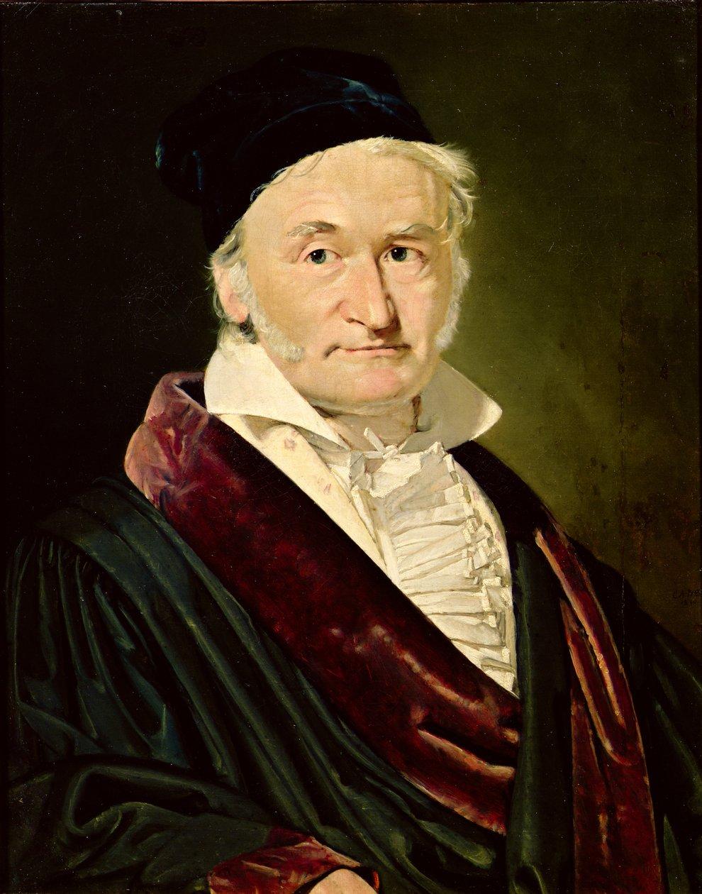
[Original image source](https://www.meisterdrucke.it/stampe-d-arte/Christian-Albrecht-Jensen/175614/Ritratto-di-Carl-Friedrich-Gauss%2C-1840.html)
**Carl Friedrich Gauss(1777—1855)**
A German mathematician and astronomer.
In *Theoria Motus Corporum Coelestium* (1809), he discussed celestial orbits and observational errors, and established an important connection between normally distributed errors and least-squares estimation.
Legendre had already published the method of least squares in 1805; Robert Adrain independently studied the normal law of errors in 1808. Simply attributing the discovery of the normal distribution to Gauss alone therefore misrepresents its mathematical history. 〔[27](#ref-turn234816search6), [29](#ref-turn523153search1), [30](#ref-turn234816search7)〕
Yet Gauss's argument contains an idea that deserves close attention:
Why, when repeatedly measuring the same unknown quantity, do we tend to use the arithmetic mean as an estimate?
For example, suppose we measure an unknown length \(\theta\) and obtain
\[
Y_1,\ldots,Y_n.
\]
Assume
\[
Y_i=\theta+\varepsilon_i,
\]
where \(\varepsilon_i\) are measurement errors.
The mathematician wants to recover \(\theta\) from these imperfect observations.
A natural method is to average:
\[
\widehat\theta=\frac1n\sum_{i=1}^nY_i.
\]
But why should the average be the right estimate?
Can we reverse the question?
**If we require the arithmetic mean to be the most likely estimate, what form must the probability distribution of the errors take?**
> Reading route: Returning to Gauss's problem of errors and estimation gives another historical source of the Gaussian law; it does not imply that Gauss worked after the modern characteristic-function proof. The functional-equation argument below is a modern reconstruction. The linearity of measurable additive functions remains a tool to be supplied later, and the related regularity questions are retained in the review issue register.
### 3.7.1 Recovering a Probability Distribution from an Optimal Estimate
Assume the errors \(\varepsilon_i\) are independent and identically distributed, with an everywhere positive, differentiable density \(f\).
Given observations \(y_1,\ldots,y_n\), the likelihood function for the parameter \(\theta\) is
\[
L(\theta)=\prod_{i=1}^n f(y_i-\theta).
\]
We now impose a strong assumption:
Whatever the sample and whatever its size, the arithmetic mean
\[
\overline y=\frac1n\sum_{i=1}^ny_i
\]
should be a maximum likelihood estimate.
Let us see what constraints this places on the density \(f\).
For convenience, let
\[
\psi(x)=\frac{f'(x)}{f(x)}.
\]
Differentiate the log-likelihood:
\[
\frac{d}{d\theta}\log L(\theta)
=
-\sum_{i=1}^n\psi(y_i-\theta).
\]
If the maximum occurs at \(\theta=\overline y\), the first-order condition requires
\[
\sum_{i=1}^n\psi(y_i-\overline y)=0.
\]
Let
\[
r_i=y_i-\overline y.
\]
Notice that
\[
\sum_{i=1}^nr_i=0.
\]
Our assumption therefore implies that
for every set of residuals satisfying \(\sum r_i=0\), we have
\[
\boxed{\sum_{i=1}^n\psi(r_i)=0.}
\]
First consider \(n=2\).
Taking residuals \(x,-x\) gives
\[
\psi(x)+\psi(-x)=0.
\]
Thus \(\psi\) is odd.
Next consider \(n=3\).
Take the residuals
\[
x,\quad y,\quad -(x+y).
\]
Then
\[
\psi(x)+\psi(y)+\psi(-(x+y))=0.
\]
Using oddness,
\[
\boxed{
\psi(x+y)=\psi(x)+\psi(y).
}
\]
This is Cauchy's functional equation!
Under a suitable regularity assumption, such as continuity, we have
\[
\psi(x)=cx
\]
for some constant \(c\).
But since
\[
\psi(x)=\frac{f'(x)}{f(x)},
\]
we obtain
\[
\frac{d}{dx}\log f(x)=cx.
\]
Integrating gives
\[
\log f(x)=\frac c2x^2+C.
\]
and hence
\[
f(x)=Ae^{cx^2/2}.
\]
For \(f\) to be an integrable probability density on the whole real line, we must have
\[
c<0.
\]
Let
\[
c=-\frac1{\sigma^2},
\]
Then
\[
f(x)=Ae^{-x^2/(2\sigma^2)}.
\]
Normalization gives
\[
\boxed{
f(x)=
\frac1{\sqrt{2\pi}\sigma}
e^{-x^2/(2\sigma^2)}.
}
\]
Once again, we have obtained the normal density!
This time, however, it did not arise as a limit of binomial coefficients.
It arose from a requirement on an estimation method:
**In the independent, identically distributed error model above, under the stated regularity conditions, requiring the arithmetic mean to be a maximum likelihood estimate for every sample leads to normally distributed errors.**
This is a modern reconstruction of Gauss's line of reasoning in 1809. It does not prove that all real-world observational errors are normally distributed; it shows a special relationship between a certain optimality requirement for the average and the normal model. 〔[30](#ref-turn234816search7)〕
Going further, we can understand why least squares is so closely connected with the normal distribution.
In the normal error model, apart from constants independent of \(\theta\) and a positive scaling factor, the negative log-likelihood is precisely
\[
\sum_{i=1}^n(y_i-\theta)^2.
\]
Maximizing the likelihood is the same as minimizing the squared error.
Thus
\[
\boxed{
\text{normal error model}
\Longrightarrow
\text{least squares and maximum likelihood are connected}.
}
\]
Mathematical methods that arose historically from different problems acquire a unified explanation here.
---
## 3.8 Must Every Random Phenomenon Eventually Become Normally Distributed?
By this point, the normal distribution may seem capable of everything.
The sum of coin tosses approaches a normal distribution.
Standardized sums of general independent random variables also approach a normal distribution.
The analysis of measurement errors again produces the normal density.
Should we conclude that the normal distribution is the inevitable final form of random phenomena?
No.
The central limit theorem has very specific assumptions.
When those assumptions fail, its conclusion may be entirely different.
Let us consider a particularly important example.
> Dependencies on later theory: This example still uses as known results the characteristic-function formula and the identification of distributions by characteristic functions. The calculation and uniqueness theory are scheduled for Chapter 11; presenting a counterexample here does not mean that the corresponding theory has already been established.
### 3.8.1 The Cauchy Distribution: A Random Variable That Averaging Cannot Tame
Let
\[
X_1,X_2,\ldots
\]
be independent and identically distributed, each with the standard Cauchy distribution:
\[
f(x)=\frac1{\pi(1+x^2)}.
\]
Its characteristic function is
\[
\phi_X(t)=e^{-|t|}.
\]
Now calculate the sample average
\[
\overline X_n=\frac1n\sum_{i=1}^nX_i.
\]
Using characteristic functions and independence,
\[
\begin{aligned}
\phi_{\overline X_n}(t)
&=
\prod_{i=1}^n
\phi_X\left(\frac tn\right)\\
&=
\left(e^{-|t|/n}\right)^n\\
&=e^{-|t|}.
\end{aligned}
\]
This is exactly the characteristic function of a single \(X_i\).
Consequently,
\[
\boxed{
\overline X_n\overset d=X_1
}
\]
for every \(n\ge1\).
This means that
no matter how many independent standard Cauchy random variables we average, the distribution of the average does not become more concentrated.
It remains standard Cauchy.
The usual convergence conclusion of the law of large numbers fails here, and the standard central limit theorem with finite variance certainly does not apply.
The reason is that the Cauchy distribution has neither a finite first absolute moment nor a finite variance.
We now see that
**the universality of the normal distribution is conditional.**
It depends on the tail behavior of the random variables, their dependence structure, and the scale chosen for summation.
When these conditions change, the limit may belong to a completely different family of distributions.
This leads to stable distributions, generalized central limit theorems, and modern probability theory's study of heavy tails.
It also shows that the normal distribution is the starting point of a broader theory of random limits, rather than the endpoint of randomness.
---
# Chapter 3 Conclusion: What Have We Really Discovered?
Let us retrace the chapter's line of thought.
At the outset, we had a very concrete difficulty:
calculating
\[
2^{-n}\sum_{k=a}^{b}\binom nk
\]
becomes exceedingly troublesome when \(n\) is large.
To understand it, we studied the central term and then compared neighboring binomial coefficients.
Taking logarithms and applying a Taylor expansion brought out
\[
e^{-x^2/2}.
\]
To obtain a nontrivial limiting shape, we had to introduce a scale such as \(\sqrt n\).
As the discrete lattice spacing tends to zero, sums of binomial coefficients become integrals.
The bell curve then emerges naturally.
The direction of generalization advanced by Laplace next tells us that this limiting phenomenon extends beyond binomial distributions.
Modern characteristic functions reveal the structure behind it:
\[
\left(
1-\frac{t^2}{2n}
+o\left(\frac1n\right)
\right)^n
\longrightarrow e^{-t^2/2}.
\]
After independent summation and suitable standardization, a complicated random system exhibits a universal limiting form determined by second-order structure.
Meanwhile, Gauss's analysis of measurement errors reveals connections between the normal distribution and the optimality of the arithmetic mean and least squares.
Two quite different paths of inquiry finally meet.
**Adding Many Random Events**
de Moivre → Laplace
\[
\sum X_i
\]
**Measurement Errors and Optimal Estimation**
Legendre → Gauss
\[
\min_\theta\sum(Y_i-\theta)^2
\]
**The Normal Distribution**
\[
f(x)=\frac{1}{\sigma\sqrt{2\pi}}e^{-\frac{(x-\mu)^2}{2\sigma^2}}
\]
Probabilistic limits, analytical structure, and statistical estimation come together here.
But I believe this chapter contains an idea more important than any individual formula.
We have found two phenomena that initially seem entirely opposed:
On the one hand, random events produce unpredictable fluctuations.
On the other, after enough accumulation, those fluctuations exhibit a stable and universal mathematical regularity.
This does not mean that the world has ceased to be random.
Quite the contrary.
**By studying randomness itself carefully, mathematicians discovered the order that randomness allows.**
We can now explain why random errors from different sources may produce approximately the same bell curve.
Yet another question arises.
In our earlier study of random variables, we could often begin by explicitly writing down their probability distributions.
But many random objects in the real world vary continuously.
For example, a particle keeps moving in a liquid.
We want to know not only its position at a particular time, but also how it moves randomly over an entire time interval.
More puzzling still:
If we observe this motion on shorter and shorter time scales, what will we ultimately see?
As the time interval tends to zero, can we construct a mathematical process that is truly continuous yet remains random throughout?
This will force us to move from individual random variables to stochastic processes consisting of infinitely many random variables.
It will also bring us back to a question that first appeared in Chapter 1:
**When the possible random outcomes form an infinite and complicated space, how should we define probability?**
This prepares the way for our journey into measure theory, stochastic processes, and Brownian motion.
---
Coming Next
## Chapter 4: When Randomness Enters Time—From Random Walks to Brownian Motion
We will begin with a very simple model:
\[
S_n=X_1+\cdots+X_n,
\qquad P(X_i=1)=P(X_i=-1)=\frac12.
\]
Then we will ask:
Why, after shrinking space by \(1/\sqrt n\) and time by \(1/n\), can a random motion that jumps on an integer lattice converge to a stochastic process with continuous paths?
This will be our first real encounter with **random functions themselves**, beyond random numbers alone.
It will also provide another important foundation for our later study of random trees, the CRT, and continuous random geometry.
The Mathematics of Chance · Volume I, Chapter 3 · Working Draft v0.1
---
# The Mathematics of Chance
Volume I · Can Chance Be Calculated?
# Chapter 4: When Randomness Enters Time—From Random Walks to Brownian Motion
Can snapshots of Gaussian distributions be assembled into a genuine random path?
In Chapter 3, we discovered a profound phenomenon in probability theory.
After suitable centering and standardization, the sum of many independent random variables may converge to a normal distribution:
\[
\frac{X_1+\cdots+X_n-n\mu}{\sigma\sqrt n}
\xrightarrow{d}N(0,1).
\]
Until now, however, we have treated the random experiment as a whole.
We cared only about the final sum of the first \(n\) random variables.
Now suppose that, instead of observing only the final sum, we record the position of the random system at every step.
The single random variable
\[
S_n=X_1+\cdots+X_n
\]
then becomes an entire sequence of random variables:
\[
S_0,S_1,S_2,\ldots
\]
We begin to ask a new question:
**How does randomness develop over time?**
This question will take probability theory beyond individual random numbers into random paths, stochastic processes, and eventually spaces of random functions.
Along the way, we will encounter one of the most important objects in modern probability theory: Brownian motion.
---
## 4.1 A Botanist Discovers a Mathematical Problem
[Original image source](https://commons.wikimedia.org/wiki/File%3APortrait_of_Robert_Brown_Wellcome_L0011784.jpg?utm_source=chatgpt.com)
**Robert Brown(1773—1858)**
A Scottish botanist who took part in botanical exploration in Australia and also studied the microscopic structure of plants.
In 1827, while studying tiny particles in pollen, he observed their persistent, irregular motion in a liquid.
By the early nineteenth century, microscopes already allowed people to observe many structures invisible to the naked eye.
Studying pollen, Brown noticed that very small particles kept trembling and changing position even when suspended in apparently still water.
At first, this motion seemed possibly related to life.
But Brown went on to study particles of nonliving matter and found that similar motion was not confined to living materials.
It could therefore not be attributed simply to the pollen being alive.
Brown made these observations in 1827 and published his report in 1828. Others had observed similar phenomena earlier, so his important contribution was a systematic investigation of the universality of the motion among different small particles, rather than being “the first to see particles move.” 〔[31](#ref-turn360592search6), [32](#ref-turn360592search7)〕
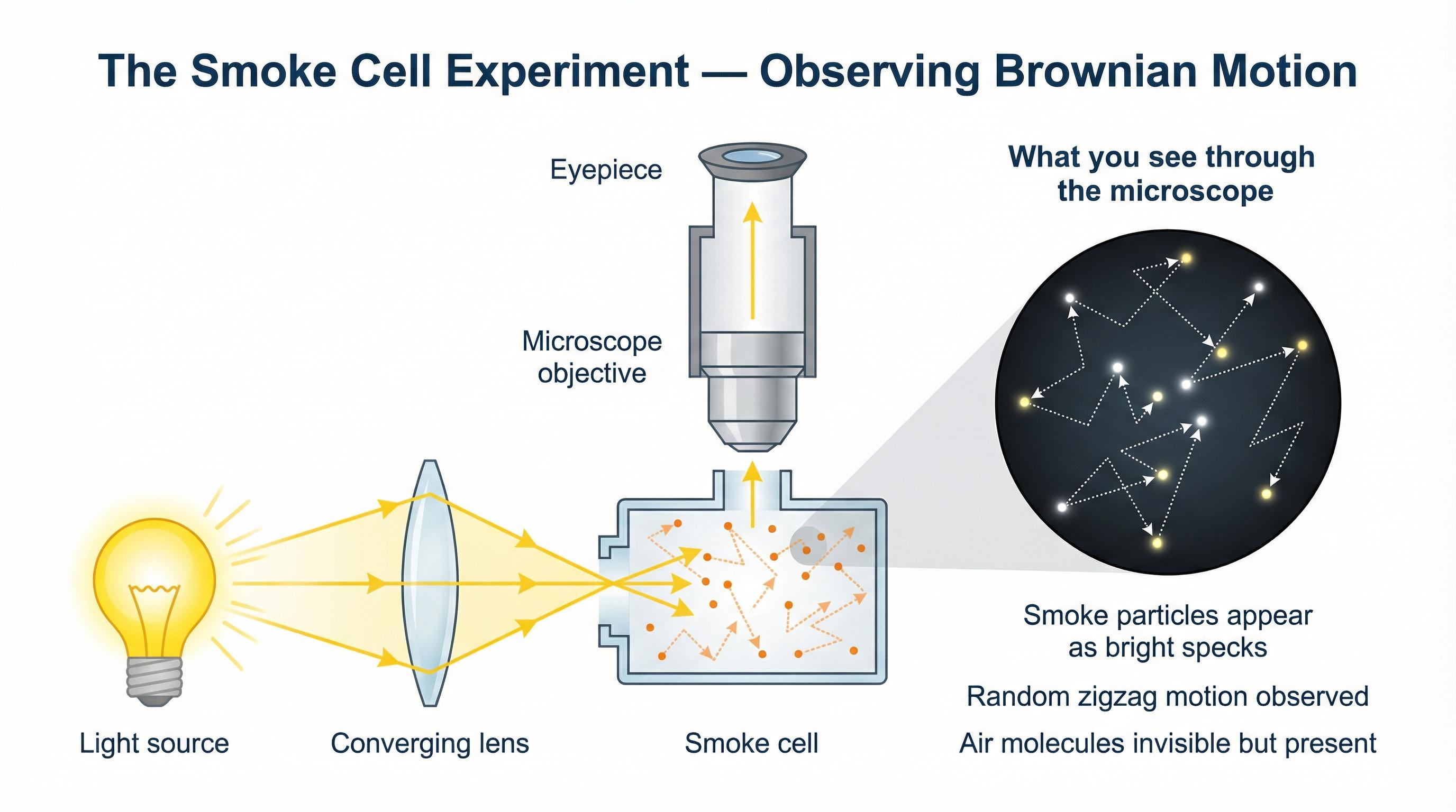
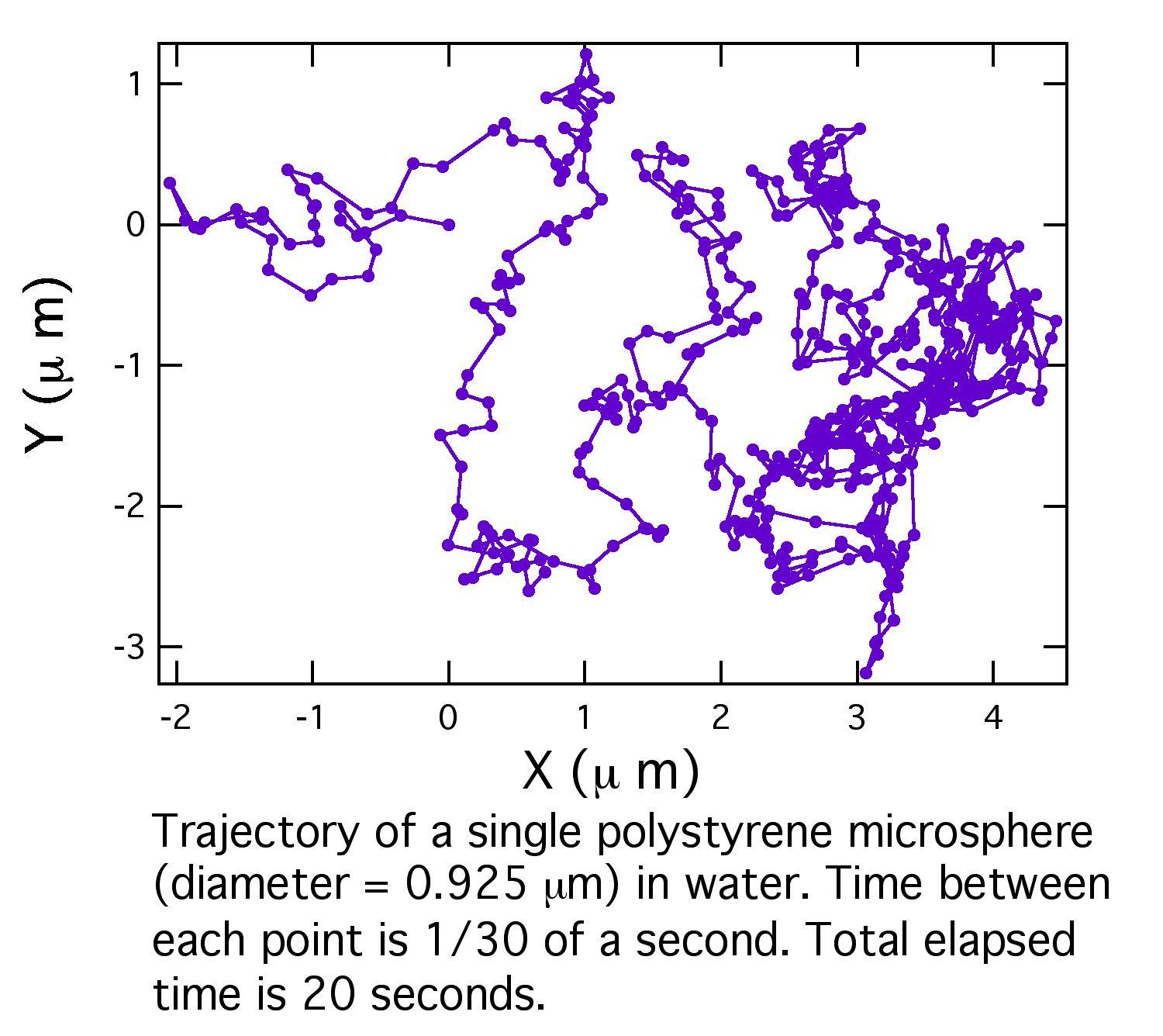
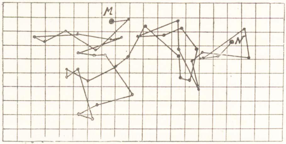
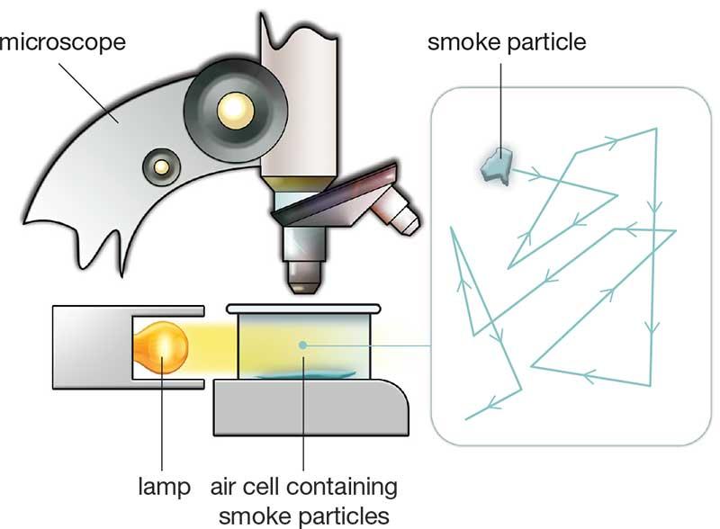
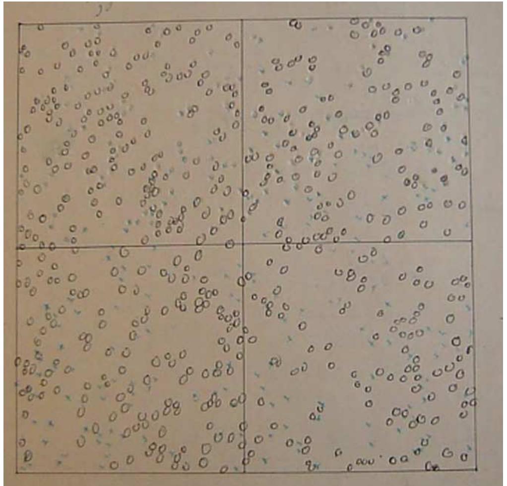
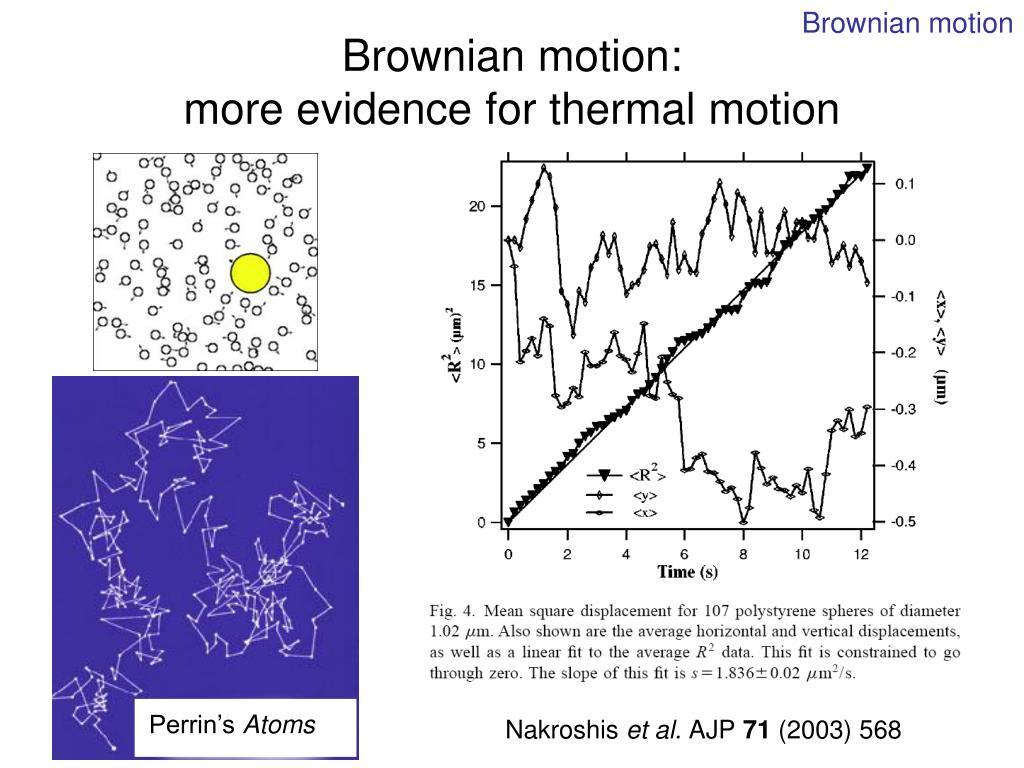
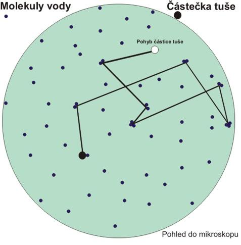
[Original image source](https://masterymind.co.uk/study-guides/physics-ocr-gcse-brownian-motion)
[Original image source](https://web.mit.edu/course/10/10.50/www/diffuse2.html)
[Original image source](https://www.heurema.com/POFQ-Perrin.htm)
[Original image source](https://www.iitianacademy.com/cie-igcse-physics-0625-particle-model-study-notes/)
[Original image source](https://www.academia.edu/4000202/_Evident_atoms_visuality_in_Jean_Perrin_s_Brownian_motion_research_Studies_in_the_History_and_Philosophy_of_Science_39_2008_312_322)
[Original image source](https://www.slideserve.com/darrius/introduction-to-the-experiments-of-physics-407)
[Original image source](https://www.mvp.cufo.cz/materialy/9.html)
Let us try to think from the perspective of an observer at the time.
If the water is still and the particle cannot move under its own power, why does it keep moving?
If some invisible microscopic action continually pushes these particles, can countless tiny motions that we cannot directly observe produce statistical laws measurable at a macroscopic scale?
This question later became closely connected with the kinetic theory of molecules, evidence for the existence of atoms, and statistical physics.
In 1905, Einstein gave a quantitative theory of the diffusion of suspended particles; Smoluchowski proposed a related theory in 1906. Jean Perrin's subsequent experiments provided important support for the predictions. 〔[33](#ref-turn360592search3), [34](#ref-turn360592search4), [35](#ref-turn360592search5)〕
There is also a historical episode worth noticing.
Before the physical theory of Brownian motion had matured, the French mathematician Louis Bachelier studied a similar continuous random price model in his 1900 financial mathematics thesis *Théorie de la spéculation*.
The rigorous probabilistic foundations of this continuous stochastic process are closely associated with Norbert Wiener's work in the 1920s, particularly in 1923.
Today, mathematical standard Brownian motion is also called the Wiener process. 〔[36](#ref-turn360592search8), [37](#ref-turn360592search0)〕
But that history came later.
To understand how such a process arises, we must first set aside continuous time, continuous paths, and even the normal distribution.
We begin with the smallest possible model.
---
## 4.2 A Particle That Can Move Only Left or Right at Each Step
Imagine a particle on the integer line.
It starts at the origin.
At each unit of time, it randomly moves one unit to the right or left.
Let
\[
\xi_1,\xi_2,\ldots
\]
be independent, identically distributed random variables with
\[
P(\xi_i=1)=P(\xi_i=-1)=\frac12.
\]
Define
\[
S_0=0,\qquad
S_n=\sum_{i=1}^n\xi_i.
\]
Then
\[
S_n
\]
is the particle's position after \(n\) steps.
This is the one-dimensional simple symmetric random walk.
We already have most of the knowledge needed to study this model.
Since
\[
\mathbb E[\xi_i]=0,
\qquad
\operatorname{Var}(\xi_i)=1,
\]
we have
\[
\boxed{
\mathbb E[S_n]=0,\qquad
\operatorname{Var}(S_n)=n.
}
\]
and hence
\[
\mathbb E[S_n^2]=n.
\]
If we measure the typical distance from the origin by the root-mean-square displacement, then
\[
\boxed{
\sqrt{\mathbb E[S_n^2]}=\sqrt n.
}
\]
This is rather strange.
If the particle always moves right, its distance from the origin after \(n\) steps is \(n\).
But when independent, symmetric randomness determines its direction, its root-mean-square displacement is only \(\sqrt n\).
Displacement scales for random walks and deterministic motion
The displacement scale of random motion is thus quite different from that of deterministic motion at constant speed.
Motion at constant speed satisfies
\[
x(t)\propto t.
\]
In this random-walk model, however, the typical displacement satisfies
\[
|S_n|_{\mathrm{typical}}\propto\sqrt n.
\]
Of course, an individual random trajectory may deviate enormously.
\(\sqrt n\) is not a deterministic bound that holds for every sample path.
It is first of all a statistical scale supplied by the second moment.
But this scale will become the key to understanding continuous random motion.
## 4.3 What Becomes of a Random Walk as Time Is Divided More Finely?
Let us pose a thought experiment.
Suppose we no longer want the particle to move once per second.
Instead, let it move \(n\) times in one second.
Each move then takes time
\[
\Delta t=\frac1n.
\]
At the same time, shrink the spatial length of each step to
\[
\Delta x=\frac1{\sqrt n}.
\]
In time \(t\), the particle then takes approximately \(nt\) steps.
The variance of its total displacement is therefore approximately
\[
nt\cdot\frac1n=t.
\]
This means that
even as individual steps shrink and the number of steps per unit time grows, the total displacement retains a nontrivial variance.
We get neither a completely stationary particle nor a system that diverges infinitely in finite time.
Now define
\[
\boxed{
W_n(t)=\frac{S_{\lfloor nt\rfloor}}{\sqrt n},
\qquad t\ge0.
}
\]
Here \(\lfloor nt\rfloor\) denotes the largest integer no greater than \(nt\).
This is the random walk after simultaneous rescaling of time and space.
Let us observe how it changes.
A scaling experiment for discrete random walks. Number of time steps: 16, 32, 64, 128, 256. Illustrative simulation: each step has length \(1/\sqrt n\) and each time interval is \(1/n\). To aid comparison, different-length prefixes of the same pregenerated sequence of random increments are used; the figure does not rigorously depict successive approximations of one and the same path.
As \(n\) increases, the original large jumps become smaller and more densely spaced.
We begin to expect that, in some limiting sense, this process will form a continuous random path.
But this immediately raises two mathematical questions.
First, does such a limit really exist?
Second, even if it exists, in what sense should we understand convergence of an entire random path?
The central limit theorem so far describes only how the distribution of a single random variable converges.
Now we want an entire function to converge:
\[
t\longmapsto W_n(t).
\]
This distinction will be crucial.
## 4.4 Why Must the Spatial Scale Be the Square Root of the Time Scale?
Let us avoid assuming that the scaling exponent is \(1/2\).
Suppose time is still shrunk by \(1/n\), but the spatial step is
\[
n^{-\alpha}
\]
where \(\alpha>0\).
Define
\[
W_n^{(\alpha)}(t)
=
n^{-\alpha}S_{\lfloor nt\rfloor}.
\]
Since
\[
\operatorname{Var}(S_{\lfloor nt\rfloor})=\lfloor nt\rfloor,
\]
we have
\[
\operatorname{Var}(W_n^{(\alpha)}(t))
=
n^{-2\alpha}\lfloor nt\rfloor.
\]
For fixed \(t>0\), the asymptotic scale is
\[
t n^{1-2\alpha}.
\]
Three quite different cases arise.
If
\[
\alpha>\frac12,
\]
then
\[
\operatorname{Var}(W_n^{(\alpha)}(t))\to0.
\]
The random displacement tends to zero in probability, giving a degenerate limit.
If
\[
\alpha=\frac12,
\]
then
\[
\operatorname{Var}(W_n^{(\alpha)}(t))\to t.
\]
the fluctuations retain a finite, nonzero scale in the limit.
If
\[
\alpha<\frac12,
\]
the variance tends to infinity. For this symmetric random walk, the central limit theorem further shows that, for any fixed \(M>0\),
\[
P(|W_n^{(\alpha)}(t)|\le M)\to0.
\]
The distributions at a fixed time therefore do not form a tight family of probability distributions on the real line.
Thus only
\[
\boxed{\alpha=\frac12}
\]
can give us the nondegenerate diffusion limit we seek.
This choice of scale is profound.
\[
\boxed{
\text{time scale}\sim\varepsilon^2,
\qquad
\text{space scale}\sim\varepsilon.
}
\]
It differs from deterministic motion at constant speed, where
\[
\text{space scale}\sim\text{time scale}.
\]
In random diffusion, time and space obey a quadratic relationship.
When we later study scaling limits of random trees, the CRT, and other continuous random geometric objects, we will encounter this idea again:
**Finding the right scaling exponent is often the first step toward discovering the limiting object.**
The actual exponent, however, depends on the random structure of the model. Not every random system must have the Brownian exponent \(1/2\).
---
## 4.5 The Central Limit Theorem Sees Only One Time
Return to
\[
W_n(t)=\frac{S_{\lfloor nt\rfloor}}{\sqrt n}.
\]
First fix a time \(t>0\).
Since
\[
S_{\lfloor nt\rfloor}
=
\xi_1+\cdots+\xi_{\lfloor nt\rfloor},
\]
the central limit theorem gives
\[
\frac{S_{\lfloor nt\rfloor}}{\sqrt{\lfloor nt\rfloor}}
\xrightarrow d N(0,1).
\]
Thus
\[
W_n(t)
=
\frac{S_{\lfloor nt\rfloor}}{\sqrt{\lfloor nt\rfloor}}
\sqrt{\frac{\lfloor nt\rfloor}{n}}.
\]
Since
\[
\frac{\lfloor nt\rfloor}{n}\to t,
\]
we obtain
\[
\boxed{
W_n(t)\xrightarrow d N(0,t).
}
\]
If a continuous-time limit exists, we see that its position at each fixed time \(t\) should therefore be normally distributed with mean 0 and variance \(t\).
Its density should thus be
\[
\boxed{
p_t(x)
=
\frac1{\sqrt{2\pi t}}
\exp\left(-\frac{x^2}{2t}\right).
}
\]
But notice:
This conclusion describes only a single fixed time.
It says nothing about the relationship between the positions at \(t=1\) and \(t=2\), or where the particle travels between those times.
A stochastic process is much more than a separate probability distribution at each time.
### 4.5.1 Why Is Knowing the Distribution at Every Time Insufficient?
Consider two stochastic processes.
The first is
\[
X_t=\sqrt t\,Z,
\]
where
\[
Z\sim N(0,1).
\]
Then, for each \(t>0\),
\[
X_t\sim N(0,t).
\]
Temporarily denote the second process by \(B_t\), and require it also to satisfy
\[
B_t\sim N(0,t).
\]
The two processes therefore have the same distribution at each fixed time.
For the first process, however,
\[
X_s=\sqrt{\frac st}X_t
\qquad(0 Using characteristic functions to pass from limits of increments to the joint vector limit invokes the multivariate continuity theorem for characteristic functions and preservation of convergence in distribution by continuous linear maps. These will be developed systematically in Chapters 11 and 13, with the language of convergence introduced in Chapter 7. Appendix F retains the product-factorization calculation. This section establishes the finite-dimensional limit conditional on those tools; it does not establish a path limit theorem.
### 4.5.3 The Covariance Structure Emerges Naturally
From
\[
B_t=B_s+(B_t-B_s),
\qquad s0\) corresponds to the process \(\sqrt{2D}\,B_t\). This explains why we study both the particle's random trajectory and the deterministic evolution of its distribution over time.
Verifying that the Gaussian density satisfies the heat equation does not replace a proof that continuous random paths exist. A density describes the distribution at each time; how a path connects those times remains the open question. For semigroups, generators, and deeper connections to stochastic calculus, continue with [semigroups and generators](#advanced-semigroup).
## 4.9 When “It Happened at Some Time” Becomes an Event
If a particle ends up near the origin, can we say it never traveled far?
Of course not. It might have crossed a high horizontal line and then returned. The final position gives only the last snapshot; “having crossed” requires the entire path.
Assume we already have a continuous Brownian path, and ask on \([0,1]\):
\[
A=\left\{\omega:\sup_{0\le t\le1}B_t(\omega)>1\right\}.
\]
This set contains a whole collection of functions with a particular history, rather than a sequence of possible die scores. We want to write \(P(A)\), but first must answer: which sets of paths may be assigned probabilities, and why does \(A\) belong among them?
Continuity offers a clue. If a continuous path is strictly above 1 at some time, it is also above 1 at a nearby rational time. Thus, for continuous paths,
\[
\left\{\sup_{0\le t\le1}B_t>1\right\}
=\bigcup_{q\in\mathbb Q\cap[0,1]}\{B_q>1\}.
\]
The right-hand side needs only countably many observation times. Here the equality is understood path by path in the continuous path space; if the process is only almost surely continuous, the equality holds on the same probability-one continuity event. Both continuity and the strict inequality matter; the reasoning cannot be applied unconditionally to the earlier random spike. We have not yet used the equality to calculate the probability, but it already indicates which set operations should continue to yield meaningful events when describing entire paths.
Our language must accommodate complements, countable unions, and limits; it must also explain why the maximum of a continuous function can serve as a random quantity. Chapter 5 begins with the sets we may discuss, Chapter 6 develops integration as a language for averaging functions, and Chapter 7 proceeds to different kinds of random convergence. Only then will we be ready to return to Brownian motion and complete the construction and path limits.
## Chapter 4 Conclusion: We Know Where the Particle Is, but Not Which Path It Took
Let us return to the microscope.
The particles Brown observed are still moving constantly in the water. Their positions keep changing and their directions seem patternless; even a clear view of a particle's present position cannot predict where it will move next.
To understand this motion, we began with the simplest random walk: each step goes left or right, independently and with equal probability. One step alone cannot reveal the scale of motion over a long period. But when many jumps are combined, cancellations between directions leave a stable scale. Quadrupling the number of steps only doubles the root-mean-square displacement.
As jumps become more frequent and steps become smaller, we therefore cannot rescale time and space arbitrarily. For random motion to persist while retaining a finite scale of fluctuations, we must maintain
\[
\Delta x\sim\sqrt{\Delta t}.
\]
At this scale, the Gaussian limit of Chapter 3 reappears: at a fixed time, the particle's position distribution approaches a bell curve whose variance grows with time.
But this gives us only one snapshot.
Collecting separate snapshots at every time does not tell us how the particle moves from one position to another. The same one-time distributions can arise from very different motions. We must turn to joint structure across times and to increments over adjacent time intervals, until independence and Gaussian distributions together give the special covariance kernel:
\[
K(s,t)=\min(s,t).
\]
This simple function records the connections between times: the random displacement accumulated at an earlier time becomes part of the later position, while subsequent independent increments bring fresh fluctuations.
When we turn from the trajectory of one particle to the position distribution of many particles, another regularity appears. At the standardized diffusion scale, the Gaussian density satisfies
\[
\frac{\partial p}{\partial t}
=\frac12\frac{\partial^2p}{\partial x^2}.
\]
The irregular motion seen under the microscope connects here with the deterministic heat equation. Individual trajectories are hard to predict, yet the distribution of possible positions can evolve regularly.
Just as we seem to be gradually understanding the motion, however, a more fundamental question emerges.
**We know where the particle may be at a given time, but have not yet established its entire continuous random path in a rigorous probability space.**
One-time distributions do not determine relationships across time. Even when every finite-dimensional distribution is specified, existence and measurability of continuous paths cannot be skipped. Our definition of Brownian motion describes the properties this motion should possess, but we must still prove that these requirements can be realized together.
In studying motion, we often care about more than the final snapshot. Has the particle ever reached a given height? Can it remain in a region throughout an interval? When does it first reach a given position?
All these questions depend on the entire path. Returning near the origin at the end does not erase the long journey a particle may have made.
The outcome of a random experiment can therefore be an entire function. We want to group paths with the same kind of history and assign a probability to that collection; before writing that probability, we must know why such a set of paths is an event we are allowed to discuss.
The particle brings us back to the question left open in Chapter 1. Counting gave clear answers for finite games of chance. Now the possible outcomes are entire continuous functions, and the old answer is insufficient.
**How should probability be defined?**
## Toward Chapter 5: Why Does Probability Need Measure Theory?
Let us simplify the difficulty. For now, set aside choosing a random path in function space, and ask only how to choose a real number uniformly from the interval \([0,1]\).
We want the probability of an interval to equal its length. Translating a set should preserve its probability, provided it remains within the interval. Combining countably many disjoint events should give a total probability equal to the sum of their probabilities.
These requirements look natural. But can we retain them all while assigning a probability to every subset of \([0,1]\)?
If even all the sets within an interval cannot be measured this way, we have still more reason to determine exactly which sets can be events before assigning probabilities to entire collections of random paths.
The next chapter begins with this ambition and takes us to the point where it becomes impossible. To understand the particle moving ceaselessly in the water, we must first rethink what it means for an event to be measurable.
[Continue to Chapter 5](#chapter-5)
The Mathematics of Chance · Volume I, Chapter 4 · Reading Candidate with Revised Conclusion, 2026-10-26
---
# Epilogue to Volume I
Chance has not lost its uncertainty by becoming calculable. What has changed is how we look: beyond a single outcome lies a structure of possibilities; within disorderly records, a stable shape may emerge. From the gaming table to the microscope, this way of seeing has already carried probability beyond its original boundaries.
---
# Volume II · Probability in an Infinite World
Structures that let reasoning and calculation survive infinity.
Infinity enlarges the random world and changes the rules of calculation. Whether averages and limits may be interchanged, and what partial information can determine, must be understood on a new foundation.
---
# The Mathematics of Chance
Volume II · Probability in an Infinite World
# Chapter 5: The Price of an Infinite World—Why Does Probability Need Measure Theory?
When people tried to measure every set, they eventually discovered that not every set can possess the kind of size we would like it to have.
In the first four chapters, we traveled a long road.
At the very beginning, we had only an unfinished game of chance.
To divide the stakes fairly, we began calculating futures that had not yet happened, gradually uncovering the ideas of probability, independence, and expectation.
We then tried to learn unknown probabilities through observation, and discovered that repeated experiments can produce stable statistical laws.
Next, the normal distribution emerged from the binomial formula and the limits of sums of independent random variables.
Finally, following discrete random walks, we identified the structure that continuous Brownian motion should have, and encountered questions about paths that remained to be resolved.
Randomness now lives not only in the finitely many outcomes of a game, but also among real numbers, continuous functions, and even in infinite-dimensional spaces.
Yet there is one question we have never seriously answered.
When we write
\[
P(A)
\]
what, exactly, does this symbol mean?
For a fair die, we can say:
\[
P(A)=\frac{|A|}{6}.
\]
There are only six equally likely outcomes.
For Brownian motion, however, we can ask about an event such as
\[
A=
\left\{
\omega:
\sup_{0\le t\le1}B_t(\omega)>1
\right\}.
\]
Here \(\omega\) is no longer simply a number.
It represents one possible realization of the entire random motion.
And \(A\) contains all random paths that have crossed height 1 at some point.
Such a set is neither finite nor something we can measure by simple counting.
Yet we still want to calculate its probability.
A seemingly natural idea therefore suggests itself:
> Since probability measures the size of a set, why not first build a mathematical theory capable of measuring the size of any set, and then apply it to random phenomena?
This looks like a purely technical problem.
As we shall discover, however, it conceals a mathematical impossibility.
---
## 5.1 A Random Experiment That Seems as Simple as Possible
Suppose we choose a real number at random from the interval \([0,1]\).
To avoid using probabilistic language before defining it, let us provisionally call this experiment a “uniform choice.”
By this we mean that the chance of the number falling in an interval should be proportional to that interval’s length.
For example:
\[
P\left(X\in\left[0,\frac12\right]\right)=\frac12,
\]
\[
P\left(X\in\left[\frac14,\frac34\right]\right)=\frac12.
\]
More generally, for
\[
0\le a0\).**
Since we add the same positive number countably infinitely many times,
\[
\sum_{q\in Q_0}c=\infty.
\]
Therefore
\[
m\left(\bigcup_{q\in Q_0}(V+q)\right)=\infty.
\]
But this union is also contained in \([-1,2]\).
By interval length,
\[
m([-1,2])=3.
\]
so its measure can be at most 3.
Thus
\[
\infty\le3.
\]
Again, a contradiction.
Whether \(m(V)=0\) or \(m(V)>0\), we reach a contradiction.
We have therefore proved:
\[
\boxed{
\begin{gathered}
\text{There is no measure defined on }\mathcal P(\mathbb R)\text{ that is}\\
\text{translation invariant、countably additive、}\\
\text{and agrees with interval length。}
\end{gathered}
}
\]
This is the core of the Vitali nonmeasurable-set argument.〔[50](#ref-turn701804search35), [51](#ref-turn701804search39)〕
### 5.3.4 Where, Exactly, Did We Fail?
What makes this proof especially striking is that it involves no particularly complicated calculation.
We performed only three operations:
Choosing representatives.
Translating sets.
Adding the sizes of disjoint sets.
Each step seems natural.
Together, however, they produce an unavoidable contradiction.
This means that some of our original wishes cannot all be fulfilled.
If we insist on interval length, translation invariance, and countable additivity, we must surrender one requirement:
**We must not require every subset of the real numbers to be assigned a measure.**
Of course, we must understand this conclusion precisely.
It does not mean that no probability space can assign probabilities to all subsets. For example, a Dirac measure concentrating all probability at a single point can perfectly well be defined on \(\mathcal P(\mathbb R)\).
What is impossible is to define on all subsets the particular kind of measure we seek, compatible with uniform length.
This distinction matters, because it tells us:
**Measurability is not an absolute property of a set, independent of a system of measure. It is closely tied to the measure structure we choose.**
We now face a new question.
If we cannot measure every set, which sets should we measure?
This leads us to \(\sigma\)-algebras.
---
## 5.4 Why Did Mathematicians Need to Invent \(\sigma\)-Algebras?
Suppose we decide to abandon the demand to measure every subset.
We select only some sets and assign probabilities to them.
Collect these sets that we permit ourselves to measure into a family, denoted by
\[
\mathcal F\subseteq\mathcal P(\Omega).
\]
What properties should \(\mathcal F\) have?
Let us not rush to a definition.
Instead, reconsider the most basic logical relationships among probabilistic events.
If an event \(A\) can be assigned a probability, then “\(A\) does not occur” should also be an event we can discuss.
Thus
\[
A\in\mathcal F
\implies A^c\in\mathcal F.
\]
If two events \(A,B\) can both be measured, then “\(A\) or \(B\) occurs” should also be measurable.
We therefore want
\[
A,B\in\mathcal F
\implies A\cup B\in\mathcal F.
\]
But in infinite random experiments, taking the union of just two events is insufficient.
For example:
Will a random walk return to the origin at some future time?
Let
\[
A_n=\{S_n=0\}.
\]
Then “returning to the origin at least once” is
\[
\bigcup_{n=1}^{\infty}A_n.
\]
while “returning to the origin infinitely often” is
\[
\bigcap_{m=1}^{\infty}
\bigcup_{n=m}^{\infty}A_n.
\]
Both events involve infinitely many set operations.
If our system of measurable events cannot handle them, studying the long-term behavior of random processes becomes difficult.
It is therefore natural to ask:
Whenever each \(A_n\) is a measurable event,
\[
\bigcup_{n=1}^{\infty}A_n
\]
should also be measurable.
This gives us the definition of a \(\sigma\)-algebra.
### Definition 5.1: \(\sigma\)-Algebra
Let \(\Omega\) be a nonempty set.
If a family of sets
\[
\mathcal F\subseteq\mathcal P(\Omega)
\]
satisfies:
1. \(\Omega\in\mathcal F\);
2. If \(A\in\mathcal F\), then \(A^c\in\mathcal F\);
3. If \(A_1,A_2,\ldots\in\mathcal F\), then
\[
\bigcup_{n=1}^{\infty}A_n\in\mathcal F,
\]
then \(\mathcal F\) is called, on \(\Omega\), a \(\sigma\)-algebra.
Its elements are called measurable sets.
That is the definition.
But we should now understand why it takes this form.
These are not three unrelated formal requirements.
They correspond, respectively, to:
The certainty that the experiment has some outcome.
The negation of an event.
Logical combinations of countably many events.
Furthermore, De Morgan’s law,
\[
\left(\bigcup_{n=1}^{\infty}A_n\right)^c
=
\bigcap_{n=1}^{\infty}A_n^c,
\]
immediately gives
\[
A_n\in\mathcal F\ (\forall n)
\implies
\bigcap_{n=1}^{\infty}A_n\in\mathcal F.
\]
A \(\sigma\)-algebra can therefore handle both countable unions and countable intersections.
### 5.4.1 Why Countably Many Rather Than Arbitrarily Many?
This question deserves consideration in its own right.
If finite unions are insufficient, why not simply require closure under arbitrary unions?
Suppose \(\mathcal F\) contains every singleton on the real line:
\[
\{x\}\in\mathcal F,
\qquad x\in\mathbb R.
\]
If \(\mathcal F\) is closed under arbitrary unions, then every set \(A\subseteq\mathbb R\) satisfies
\[
A=\bigcup_{x\in A}\{x\}\in\mathcal F.
\]
Hence
\[
\mathcal F=\mathcal P(\mathbb R).
\]
We have returned to the starting point that failed in Vitali’s proof.
The distinction between countable and arbitrary unions is therefore no arbitrary technical restriction invented by mathematicians.
It allows us to retain powerful limiting operations without including every subset in our measurable structure.
This is especially important in probability theory.
Random sequences indexed by the natural numbers, limiting unions and intersections, and many events concerning paths of stochastic processes can all be expressed through countably many operations.
An arbitrary uncountable union, however, need not be measurable.
This will influence our methods when we later handle continuous-time stochastic processes.
---
## 5.5 Is Having More Measurable Events Always Better?
Now imagine two \(\sigma\)-algebras
\[
\mathcal F_1\subseteq\mathcal F_2.
\]
If we regard them as collections of distinguishable events, \(\mathcal F_2\) allows us to distinguish more possibilities.
This suggests an interpretation of great importance in modern probability:
**A \(\sigma\)-algebra can be viewed as a structure of information.**
For example, before tossing a coin, we consider only the certain event and the impossible event:
\[
\mathcal F_0=\{\varnothing,\Omega\}.
\]
After the toss, if the outcome space is
\[
\Omega=\{H,T\},
\]
we can distinguish heads from tails:
\[
\mathcal F_1=\mathcal P(\Omega).
\]
Thus
\[
\mathcal F_0\subseteq\mathcal F_1.
\]
The latter contains more distinguishable events.
Of course, “measurable events” cannot in every setting be directly identified with “what an observer actually knows.” This is a mathematical interpretation, which we will later make precise through conditional expectation and filtrations.
Yet it already anticipates an important idea:
When studying a stochastic process, we must ask not only what happened, but also **how much information about the random world we have acquired at a given time**.
This gives rise to increasing families of \(\sigma\)-algebras:
\[
\mathcal F_s\subseteq\mathcal F_t,
\qquad s\le t.
\]
These will form the foundation of martingale theory.
The abstract families of sets introduced here will therefore do more than ensure that probability is rigorously defined: they will directly describe how information grows over time.
This will become especially important in the chapter on conditional expectation.
---
## 5.6 Borel Sets: How Can the Simplest Sets Generate a Rich Enough Measurable World?
We can now finally answer:
If we cannot measure every subset of the real numbers, which sets should we at least measure?
Intervals remain the most natural starting point.
They have clear geometric lengths.
We therefore first require every open interval to be measurable.
Then, as discussed in the previous section, whenever sets are measurable, their complements, countable unions, and countable intersections should also be measurable.
A construction problem emerges:
**Starting from all open intervals and repeatedly performing these permitted set operations, what can we obtain?**
To express this rigorously, first introduce the notion of generation.
Given a family of sets \(\mathcal C\subseteq\mathcal P(\Omega)\), define
\[
\boxed{
\sigma(\mathcal C)
=
\bigcap\left\{
\mathcal F:
\mathcal F\text{ is a }\sigma\text{-algebra},
\ \mathcal C\subseteq\mathcal F
\right\}.
}
\]
Because an arbitrary intersection of \(\sigma\)-algebras remains a \(\sigma\)-algebra, this definition does indeed produce, among the families containing \(\mathcal C\), the smallest \(\sigma\)-algebra.
We say that \(\mathcal C\) generates this \(\sigma\)-algebra.
Now let \(\mathcal O\) be the family of all open sets in \(\mathbb R\).
Define
\[
\boxed{
\mathcal B(\mathbb R)=\sigma(\mathcal O).
}
\]
This is the Borel \(\sigma\)-algebra on the real line.
It contains open sets, closed sets, and every set obtainable through countable unions, intersections, and complementation.
One very useful fact is:
\[
\boxed{
\mathcal B(\mathbb R)
=
\sigma\bigl(\{(a,b):a,b\in\mathbb Q,\ a0\), we can choose for each \(A_k\) an open-interval cover whose total length does not exceed
\[
m^*(A_k)+\frac{\varepsilon}{2^k},
\]
Here we first suppose that the relevant outer measures are finite; if any term is infinite, the desired inequality holds immediately.
Combining all these covers gives an open-interval cover of \(\bigcup_kA_k\).
Hence
\[
m^*\left(\bigcup_{k=1}^{\infty}A_k\right)
\le
\sum_{k=1}^{\infty}m^*(A_k)+\varepsilon.
\]
Letting \(\varepsilon\downarrow0\) gives
\[
\boxed{
m^*\left(\bigcup_{k=1}^{\infty}A_k\right)
\le
\sum_{k=1}^{\infty}m^*(A_k).
}
\]
This is the upper bound for countable additivity, or **countable subadditivity**.
Notice that we obtain an inequality, not an equality.
Outer measure therefore already assigns some nonnegative generalized size to **every subset of the real numbers**.
But it does not guarantee countable additivity for all disjoint sets.
This is unsurprising.
Vitali’s theorem has already told us that if outer measure preserves translation invariance and interval length, it cannot be countably additive on all subsets.
The problem has therefore changed.
We already have an outer measure defined on every subset.
Now we must find the sets on which outer measure behaves like a genuine measure.
This gives another natural origin for measurability.
## 5.8 Carathéodory: Which Sets Should We Permit Ourselves to Measure?
> Editorial supplement: Appendix A gives expanded proofs of closure under finite unions, closure under countable unions, and countable additivity; Appendix B treats the cut points in open covers.
Consider an arbitrary set \(A\subseteq\mathbb R\).
Suppose we divide another set \(E\) into two parts:
\[
E\cap A
\]
and
\[
E\setminus A.
\]
These are plainly disjoint, and
\[
E=(E\cap A)\cup(E\setminus A).
\]
By subadditivity of outer measure, we always have
\[
m^*(E)
\le
m^*(E\cap A)+m^*(E\setminus A).
\]
But if \(A\) is truly compatible with the notion of length, we seem entitled to expect more:
Dividing any set \(E\) according to membership in \(A\) should not change the total outer measure out of nowhere.
In other words, we want
\[
m^*(E)
=
m^*(E\cap A)+m^*(E\setminus A).
\]
Notice a crucial detail here.
**We do not ask merely that this equality hold when \(E=\mathbb R\) or \(E=A\); we require it for every set \(E\).**
This is the idea behind Carathéodory’s criterion for measurability.
### Definition 5.2: Carathéodory Measurable Set
Given the outer measure \(m^*\), if a set \(A\subseteq\mathbb R\) satisfies:
For every \(E\subseteq\mathbb R\),
\[
\boxed{
m^*(E)
=
m^*(E\cap A)+m^*(E\setminus A),
}
\]
then \(A\) is called Lebesgue measurable.
Denote the family of all such sets by
\[
\mathcal L.
\]
At first sight, this definition looks more abstract than the definition of a \(\sigma\)-algebra.
But we already understand where it comes from.
Outer measure can measure any set, yet may fail to be additive.
We therefore seek sets that preserve the desired additive property whenever they are used to cut any other set.
In the early twentieth century, Carathéodory developed this idea into an important construction tool in the general theory of outer measure.〔[52](#ref-turn701804search6), [53](#ref-turn701804search37)〕
Now let us see where its real power lies.
### 5.8.1 Why Do These Measurable Sets Automatically Form a \(\sigma\)-Algebra?
We begin with closure properties.
Since the definition is entirely symmetric in \(A\) and \(A^c\),
\[
A\in\mathcal L
\implies A^c\in\mathcal L.
\]
Repeatedly applying the measurability equality to sets also shows that if \(A,B\in\mathcal L\), then
\[
A\cup B\in\mathcal L.
\]
More generally, let \(A_1,A_2,\ldots\in\mathcal L\).
Turn them into pairwise disjoint sets:
\[
B_1=A_1,
\]
\[
B_n=A_n\setminus\bigcup_{k=1}^{n-1}A_k,\qquad n\ge2.
\]
Each of these \(B_n\) is measurable.
Moreover,
\[
\bigcup_{n=1}^{\infty}A_n
=
\bigsqcup_{n=1}^{\infty}B_n.
\]
For any \(E\subseteq\mathbb R\), repeated finite measurable partitions give
\[
m^*(E)
\ge
\sum_{k=1}^{N}m^*(E\cap B_k)
+
m^*\left(E\setminus\bigcup_{k=1}^{\infty}B_k\right).
\]
Letting \(N\to\infty\) and using subadditivity of outer measure,
\[
m^*\left(E\cap\bigcup_{k=1}^{\infty}B_k\right)
\le
\sum_{k=1}^{\infty}m^*(E\cap B_k),
\]
we obtain
\[
m^*(E)
\ge
m^*\left(E\cap\bigcup_{k=1}^{\infty}B_k\right)
+
m^*\left(E\setminus\bigcup_{k=1}^{\infty}B_k\right).
\]
The reverse inequality already follows from subadditivity.
The two sides are therefore equal.
This proves that a countable union is still measurable.
Thus
\[
\boxed{\mathcal L\text{ is a }\sigma\text{-algebra}.}
\]
Furthermore, similar finite-partition and limiting arguments show:
If \(A_1,A_2,\ldots\in\mathcal L\) are pairwise disjoint, then
\[
\boxed{
m^*\left(\bigcup_{n=1}^{\infty}A_n\right)
=
\sum_{n=1}^{\infty}m^*(A_n).
}
\]
Consequently, restricting outer measure to \(\mathcal L\),
\[
m=m^*|_{\mathcal L},
\]
gives a genuine measure.
This is exactly what we have been seeking.
### 5.8.2 Why Are All Borel Sets Included?
One important question remains.
Can this construction at least measure intervals?
The answer is yes.
For example, consider the half-line
\[
A=(-\infty,a).
\]
For any \(E\subseteq\mathbb R\), cover \(E\) by a family of open intervals, and then split each covering interval into left and right parts at \(a\).
The lengths of the two parts still add up to the original interval’s length.
Taking the infimum over the total lengths of these covers proves
\[
m^*(E\cap A)+m^*(E\setminus A)\le m^*(E).
\]
The other direction follows from subadditivity.
Thus \(A\) is measurable.
Similarly, every open interval is measurable.
And because \(\mathcal L\) is a \(\sigma\)-algebra,
\[
\boxed{
\mathcal B(\mathbb R)\subseteq\mathcal L.
}
\]
We have thereby accomplished something very important:
Starting from interval length, we have constructed a translation-invariant, countably additive measure on a sufficiently rich family of sets.
It is Lebesgue measure.
### 5.8.3 Are Borel Sets and Lebesgue Measurable Sets the Same?
One further point is easily overlooked.
\[
\mathcal B(\mathbb R)
\subsetneq
\mathcal L.
\]
In other words, there are strictly more Lebesgue measurable sets than Borel sets.
Why?
Consider the classical middle-thirds Cantor set \(C\).
It is closed, hence Borel.
It is uncountable, but
\[
m(C)=0.
\]
because at step \(n\), the \(2^n\) remaining intervals have total length
\[
\left(\frac23\right)^n,
\]
and this length tends to zero.
More importantly, under Lebesgue measure, every subset of a null set is still measurable and has measure zero.
Indeed, if \(A\subseteq C\), then
\[
0\le m^*(A)\le m^*(C)=0.
\]
Thus \(m^*(A)=0\), and any set of outer measure zero automatically satisfies Carathéodory’s measurability criterion.
Hence
\[
\boxed{
A\subseteq C\implies A\in\mathcal L.
}
\]
But the Cantor set has the same cardinality as the reals, and its power set has strictly greater cardinality than the family of Borel sets. For the full well-founded Borel coding and cardinal comparison, see the [measure foundations](../foundations/t-measure.md#t-measure-borel-code).
There must therefore be subsets of the Cantor set that are not Borel, yet are Lebesgue measurable.
This shows that Borel measure can be completed by adjoining all subsets of null sets to the measurable structure. The [companion proof](../foundations/t-measure.md#t-measure-completion) constructs completion for an arbitrary measure and proves minimality and uniqueness.
We finally have a rigorous continuous uniform probability model:
\[
\boxed{
\begin{aligned}
\Omega&=[0,1],\\
\mathcal F&=\mathcal L|_{[0,1]},\\
P(A)&=m(A).
\end{aligned}
}
\]
where
\[
\mathcal L|_{[0,1]}
=
\{A\subseteq[0,1]:A\in\mathcal L\}.
\]
For every \(0\le a0\), then
\[
P(\mathbb N)
=
\sum_{n=1}^{\infty}c
=\infty.
\]
But we require
\[
P(\mathbb N)=1.
\]
Thus \(c>0\) is impossible.
If \(c=0\), then
\[
P(\mathbb N)
=
\sum_{n=1}^{\infty}0
=0.
\]
Again, a contradiction.
Therefore:
\[
\boxed{
\text{There is no measure defined on }\mathbb N\text{ 、}\\
\text{that is a countably additive probability measure giving equal mass to every singleton。}
}
\]
The real problem is not that there are too many natural numbers.
It is that we require all singletons to have equal probabilities while also requiring all the natural numbers together to have probability 1.
If probabilities may vary with the number, there is no difficulty.
For example:
\[
P(\{n\})=2^{-n},
\qquad n=1,2,\ldots
\]
because
\[
\sum_{n=1}^{\infty}2^{-n}=1.
\]
This deserves some reflection.
In Chapter 1, symmetry led us to uniform probabilities.
Now, however, symmetry may conflict with countable additivity.
**Not every symmetry requirement that feels fair can be realized in an infinite probability space.**
Probability theory must distinguish clearly between symmetries that produce valid probability distributions and those expressible only in other mathematical frameworks.
---
## 5.10 Kolmogorov: Probability Finally Becomes a Special Case of Measure
We now have the main mathematical structures needed to establish modern probability theory.
A space of outcomes \(\Omega\).
A family of events \(\mathcal F\) to which probabilities may be assigned.
And a function \(P\) that assigns numerical values to these events.
We can therefore finally state formally:
### Definition 5.3: Probability Space
A probability space is a triple
\[
\boxed{(\Omega,\mathcal F,P)}
\]
where:
\(\Omega\) is a nonempty sample space;
\(\mathcal F\) is, on \(\Omega\), a \(\sigma\)-algebra;
\(P:\mathcal F\to[0,1]\) satisfies
\[
P(\Omega)=1,
\]
and for any pairwise disjoint events \(A_1,A_2,\ldots\in\mathcal F\),
\[
\boxed{
P\left(\bigcup_{n=1}^{\infty}A_n\right)
=
\sum_{n=1}^{\infty}P(A_n).
}
\]
This gives the modern Kolmogorov axiomatic framework for probability.
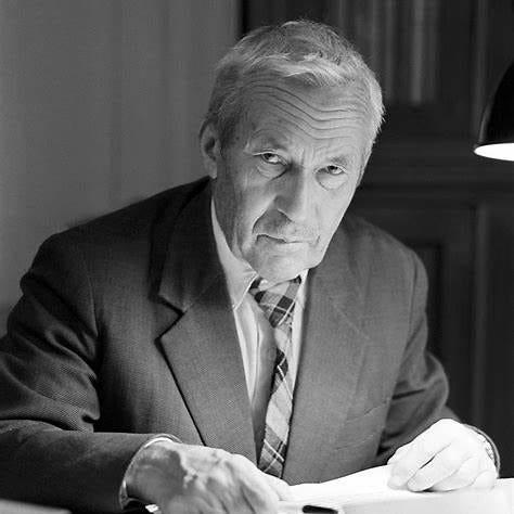
[Original image source](https://valeman.medium.com/andrey-kolmogorov-master-of-uncertainty-and-order-1080618e1afe)
**Andrey Kolmogorov(1903—1987)**
In 1933 he published *Grundbegriffe der Wahrscheinlichkeitsrechnung* (*Foundations of the Theory of Probability*), systematically establishing probability theory within the axiomatic framework of measure theory.
Here, too, we must respect history.
Kolmogorov did not first discover the connection between probability and measure in 1933. Earlier work by Borel, Lebesgue, and other mathematicians had already laid its foundations.
But Kolmogorov gave this framework a clear, systematic expression that became the basic language of modern probability.〔[48](#ref-turn701804search0), [54](#ref-turn701804search40)〕
We can finally return to the classical probability of Chapter 1 with a new understanding.
Suppose
\[
\Omega=\{\omega_1,\ldots,\omega_n\},
\]
Take
\[
\mathcal F=\mathcal P(\Omega).
\]
Define
\[
P(A)=\frac{|A|}{n}.
\]
Then all the probability axioms are satisfied.
Classical probability is therefore simply a particular example of a modern probability measure.
For a finite outcome space with unequal probabilities, we can likewise choose
\[
p_i\ge0,\qquad\sum_{i=1}^{n}p_i=1,
\]
and then define
\[
P(A)=\sum_{\omega_i\in A}p_i.
\]
For a countably infinite space, we can use a summable sequence of weights.
For a continuous space, we can use Lebesgue measure or other probability measures constructed from it.
We suddenly see:
\[
\boxed{
\begin{gathered}
\text{classical equally likely counting}\\
\text{discrete probabilities with unequal weights}\\
\text{continuous uniform probability}\\
\text{more general probability distributions}
\end{gathered}
\quad
\begin{gathered}
\\[-1.5em]
\Bigg\}\\
\\[-0.5em]
\text{probability measures}
\end{gathered}
}
\]
These mathematical objects, once handled separately, have finally been unified.
But this unification does not arise because every probability can be reduced to counting.
Quite the reverse.
**Counting is only one special form of measure.**
That is the theoretical expansion we have achieved since Chapter 1.
---
## 5.11 Why Must Random Variables Be Measurable Functions?
We now have a probability space
\[
(\Omega,\mathcal F,P).
\]
But probability theory studies more than events.
We also need random variables.
For example, when rolling three dice, we may care only about the sum of their scores:
\[
X(\omega)=\text{sum of the scores on three dice}.
\]
In a finite space, any such function can be handled directly.
In a general probability space, however, we must be more careful.
Suppose
\[
X:\Omega\to\mathbb R
\]
is a function.
If we want to study the event
\[
\{X\le a\},
\]
it is actually
\[
X^{-1}((-\infty,a]).
\]
To calculate its probability, we must require
\[
X^{-1}((-\infty,a])\in\mathcal F.
\]
Nor should we handle only interval events of this kind.
For every Borel set \(B\), we want to calculate
\[
P(X\in B).
\]
We must therefore require:
\[
X^{-1}(B)\in\mathcal F,
\qquad B\in\mathcal B(\mathbb R).
\]
This is where the measurability requirement for random variables comes from.
### Definition 5.4: Random Variable
Let \((\Omega,\mathcal F,P)\) be a probability space.
If a function
\[
X:\Omega\to\mathbb R
\]
satisfies
\[
\boxed{
X^{-1}(B)\in\mathcal F
\quad
\text{for all }B\in\mathcal B(\mathbb R),
}
\]
then \(X\) is called a real-valued random variable.
Notice that this definition makes no demand whatsoever that the values of \(X\) themselves have some special random form.
Its only requirement is:
**Borel events formulated through \(X\) must correspond to events that are permitted to be measured in the original probability space.**
Only then can we rigorously define the distribution of \(X\):
\[
\boxed{
P_X(B)=P(X^{-1}(B)).
}
\]
This is exactly the pushforward-measure structure foreshadowed by the sum of three dice in Chapter 1.
There, we merely grouped the 216 ordered outcomes according to their sums.
Now we find that the same mathematical idea works in general probability spaces.
The distribution of a random variable is the new measure produced from the original probability measure by a measurable map.
### 5.11.1 Back to Brownian Motion: Why Is the Maximum of a Continuous Path Measurable?
Do you remember the event we studied in Chapter 4?
\[
A=\left\{
\omega:
\sup_{0\le t\le1}B_t(\omega)>1
\right\}.
\]
We can finally explain rigorously why it is measurable.
Suppose Brownian motion has already been constructed as a random element taking values in \(C([0,1])\).
For every continuous function \(f\),
\[
\boxed{
\sup_{0\le t\le1}f(t)
=
\sup_{t\in\mathbb Q\cap[0,1]}f(t).
}
\]
Why?
Because the rationals are dense in \([0,1]\) and \(f\) is continuous.
Thus, although we originally take a supremum over uncountably many times, for continuous paths it suffices to take the supremum over countably many rational times.
Hence
\[
A=
\bigcup_{q\in\mathbb Q\cap[0,1]}
\{B_q>1\}.
\]
Here we use the fact that if the supremum of a collection of real numbers exceeds 1, at least one member of that collection exceeds 1.
For each rational number \(q\), the event
\[
\{B_q>1\}
\]
is measurable.
Since \(\mathbb Q\cap[0,1]\) is countable,
\[
A\in\mathcal F.
\]
We finally see:
**Closure of a \(\sigma\)-algebra under countable unions, a countable dense subset of the reals, and continuity of paths together ensure the measurability of certain complicated path events.**
Properties that seem to come from different areas of mathematics fit together very naturally here.
This also explains why, when constructing Brownian motion in Chapter 4, we could not simply specify normal distributions at each time and declare that we had a complete theory of random paths.
We also need measurability, the structure of a function space, and appropriate path regularity.
---
## 5.12 What, Exactly, Does Probability 1 Mean?
There is another term we have used repeatedly without ever explaining it carefully.
Almost surely.
For example, in Chapter 4 we said:
Brownian paths are almost surely continuous.
We also said:
Brownian paths are almost surely nowhere differentiable.
What does this mean?
We can now give a rigorous definition.
If an event \(A\in\mathcal F\) satisfies
\[
P(A)=1,
\]
we say that \(A\) occurs almost surely.
If
\[
P(A)=0,
\]
we call \(A\) a probability-zero event.
Notice that
\[
P(A)=1
\]
does not mean
\[
A=\Omega.
\]
Likewise,
\[
P(A)=0
\]
does not mean
\[
A=\varnothing.
\]
For example, in the uniform probability space on \([0,1]\),
\[
P(X\in\mathbb Q)=0.
\]
Yet the interval certainly contains many rational numbers.
Probability zero therefore does not mean logical impossibility.
And probability 1 does not mean the absence of exceptions.
This distinction will become a very important idea in modern probability.
Often, we do not need a property to hold for every sample path.
We need only prove that it holds for all outcomes outside a set of probability zero.
Thus:
\[
X_n\xrightarrow{\mathrm{a.s.}}X
\]
means
\[
P\left(
\left\{\omega:
\lim_{n\to\infty}X_n(\omega)=X(\omega)
\right\}
\right)=1.
\]
Here we encounter measurability again.
For this probability expression to be valid, the set
\[
\left\{
\omega:
\lim_{n\to\infty}X_n(\omega)=X(\omega)
\right\}
\]
must belong to \(\mathcal F\).
For measurable real-valued random variables, this is indeed true, because the convergence event can be expressed through countable unions and intersections and conditions involving rational thresholds.
Therefore, **almost sure convergence is more than a notion of limits alone: it combines pointwise convergence from analysis with the measure-theoretic idea of null sets.**
When we systematically study the various modes of convergence, this will underpin our understanding of their differences.
---
# Chapter 5 Conclusion: Why Must Mathematics Learn to Let Go?
We began with a perfectly reasonable wish.
We wanted to select a number uniformly at random from \([0,1]\) and calculate the probability of every possible event.
To do so, we tried to construct a way of measuring the size of every set.
But infinite sets forced us to reconsider the meaning of “size.”
First, cardinality cannot represent interval length.
Then we discovered that a dense set can have measure zero.
More importantly, Vitali’s construction told us:
Under the usual foundations of set theory, we cannot retain all the properties we originally wanted at once.
We therefore had to abandon the requirement that every subset be measurable.
But this restriction did not impoverish the theory.
Quite the opposite.
Through \(\sigma\)-algebras, we found a measurable structure that accommodates infinite operations on events while remaining compatible with countable additivity.
Through outer measure and Carathéodory measurability, we constructed Lebesgue measure from interval length.
Finally, Kolmogorov’s axiomatic framework unified classical probability, discrete distributions, and continuous probability.
Looking back over the entire journey:
**Counting finite outcomes**
\[
P(A)=\frac{|A|}{|\Omega|}
\]
**The problem of size in infinite sets**
Cardinality no longer coincides with length
**Vitali’s impossibility**
The required properties cannot hold simultaneously on all subsets
**Measurability and \(\sigma\)-algebras**
\[
\mathcal F\subseteq\mathcal P(\Omega)
\]
**The modern probability space**
\[
(\Omega,\mathcal F,P)
\]
Counting becomes a special case of measure
I believe what we should remember most from this chapter is more than the three axioms of a probability space.
It is a deeper idea:
**A mathematical theory sometimes matures not by granting us more and more freedom, but by revealing which freedoms must be restricted.**
We gave up the requirement to measure every set in exchange for a rigorous theory capable of handling infinity, limits, and complicated random objects.
Yet although we now possess probability measures, one central question remains unresolved.
We can calculate the probabilities of events:
\[
P(A).
\]
But given a random variable
\[
X:\Omega\to\mathbb R,
\]
how should we calculate its average?
In a finite space, this is simple:
\[
\mathbb E[X]
=
\sum_{\omega\in\Omega}X(\omega)P(\{\omega\}).
\]
For continuous distributions, we are accustomed to writing:
\[
\mathbb E[X]
=
\int_{\mathbb R}x f_X(x)\,dx.
\]
But what if a random variable has neither a discrete distribution nor a probability density?
What if its distribution mixes discrete and continuous parts?
Or what if we study a singular distribution with no density?
Must we invent a new formula for expectation for every type of distribution?
We already know that probability is measure.
Does expectation, too, have a unified mathematical form?
The answer is:
\[
\boxed{
\mathbb E[X]=\int_\Omega X\,dP.
}
\]
For now, however, this formula is only a promise waiting to be explained.
We must answer:
Why can integration unify all these averages?
How can general integrals be constructed from simple functions?
Why do some random variables lack finite expectations?
When may we move a limit inside an expectation?
These questions will lead us into the next chapter.
# Chapter 6: The Rebirth of the Average—From Weighted Sums to the Lebesgue Integral
We shall return to the fair stakes of Chapter 1.
This time, however, we will regard expectation as more than a way of calculating winnings.
We will discover:
**Why integration is the most natural extension of weighted averaging, and why measure theory ultimately needs an integral different from Riemann’s.**
The monotone convergence theorem, Fatou’s lemma, the dominated convergence theorem, and the Fubini–Tonelli theorem will gradually emerge along the way.
We will also prepare for a rigorous study of conditional expectation, martingales, and the various modes of convergence.
The Mathematics of Chance · Volume II, Chapter 5 · Working draft v0.1
---
# The Mathematics of Chance
Volume II · Probability in an Infinite World
# Chapter 6: The Rebirth of the Average—From Weighted Sums to the Lebesgue Integral
Why should a simple average of gambling winnings ultimately require an entirely new theory of integration?
In Chapter 5, we underwent a major transformation in mathematical thought.
To define probability on infinite sets, we had to abandon a seemingly natural wish: not every set can have a measure compatible with interval length.
We therefore established the probability space
\[
(\Omega,\mathcal F,P).
\]
Probability became more than “the number of favorable outcomes divided by the total number of outcomes”: it became a countably additive measure defined on a \(\sigma\)-algebra.
This finally enabled us to study continuous distributions, infinite random sequences, and complicated random objects such as Brownian motion rigorously.
Looking back over the development of probability, however, we find another mathematical concept of almost equal importance that has accompanied us throughout.
It is expectation.
In Chapter 1, we used expectation to divide the stakes fairly in an unfinished game.
In Chapter 2, we used expectation to estimate unknown parameters.
In Chapter 3, we used means and variances to study normal limits.
In Chapter 4, we even calculated the expectation of the sum of squared increments of an entire stochastic process.
But we never really answered:
**Why should expectation be defined in the familiar way? What exactly is expectation when the sample space is no longer finite?**
We now possess measure.
Perhaps it is time to understand averages afresh, from the beginning.
---
## 6.1 It Still Begins with a Fair Game of Chance
Imagine returning once more to Chapter 1.
A gambling contract has three possible payoffs:
\[
X=
\begin{cases}
10,&\text{with probability }1/2,\\
20,&\text{with probability }1/3,\\
-5,&\text{with probability }1/6.
\end{cases}
\]
If we want a single number to represent its average payoff, the most natural calculation is
\[
\begin{aligned}
\mathbb E[X]
&=10\cdot\frac12
+20\cdot\frac13
-5\cdot\frac16\\
&=\frac{65}{6}.
\end{aligned}
\]
Here we are taking a weighted sum:
\[
\boxed{
\mathbb E[X]=\sum_i x_ip_i.
}
\]
But we should examine this expression more closely.
It actually contains two entirely different mathematical objects.
The first is the payoff:
\[
x_i.
\]
The second is the probability weight associated with each payoff:
\[
p_i.
\]
Expectation is a mathematical operation combining the two.
Now write it in another form.
Let the sample space be
\[
\Omega=\{\omega_1,\omega_2,\omega_3\},
\]
and define the random variable
\[
X(\omega_1)=10,\quad
X(\omega_2)=20,\quad
X(\omega_3)=-5.
\]
with corresponding probabilities
\[
P(\{\omega_1\})=\frac12,\quad
P(\{\omega_2\})=\frac13,\quad
P(\{\omega_3\})=\frac16.
\]
Then
\[
\mathbb E[X]
=
\sum_{\omega\in\Omega}
X(\omega)P(\{\omega\}).
\]
This formula already comes very close to the idea of integration.
What we are doing, in fact, is:
Accumulating the values of a function on the sample space, weighted according to a rule for the sizes of sets.
A new question therefore arises:
**If the sample space has infinitely many outcomes, can this weighted summation be extended to some kind of integral?**
### 6.1.1 From Finite to Continuous Outcomes
Suppose the payoff is no longer restricted to three values.
From \([0,1]\), we choose a real number \(U\) uniformly at random, then receive the payoff
\[
X=U^2.
\]
Chapter 5 has already supplied a rigorous uniform probability space:
\[
\Omega=[0,1],
\qquad P=\text{Lebesgue length measure}.
\]
We want to calculate
\[
\mathbb E[U^2].
\]
From calculus, we would naturally write:
\[
\mathbb E[U^2]
=
\int_0^1x^2\,dx
=
\frac13.
\]
But this step contains an assumption we have not yet explained:
Why should the average of a continuous random variable equal an area integral of a function over an interval?
Our usual explanation is that the interval can be divided into many small pieces.
For example:
\[
0=x_0xf(x)
The rectangles’ widths come from the partition of the domain, while their heights are determined by the function values on the respective intervals.
Define a partition
\[
\mathcal P=\{a=x_0 Editorial supplement: The limit function \(f\) is also assumed nonnegative and measurable; on an incomplete space, almost everywhere convergence should be interpreted using a measurable version of the limit. See Appendix E. A proof from simple integrals without assuming general linearity is given in the [monotone-convergence companion](../foundations/t-integral.md#t-integral-mct).
Let \(f_1,f_2,\ldots\) be nonnegative measurable functions satisfying
\[
0\le f_1\le f_2\le\cdots
\]
and
\[
f_n(\omega)\uparrow f(\omega)
\]
almost everywhere.
Then
\[
\boxed{
\lim_{n\to\infty}
\int_\Omega f_n\,d\mu
=
\int_\Omega f\,d\mu.
}
\]
Both sides are permitted to equal \(+\infty\).
This theorem is exceptionally powerful.
It does not require \(\mu(\Omega)\) to be finite.
It does not require a uniform upper bound on the \(f_n\).
It does not even require their integrals to be finite.
It requires only nonnegativity and monotone increase.
Why are these two conditions so effective?
### 6.5.1 Proof: First Understand the Easy Direction
Since
\[
f_n\le f,
\]
monotonicity of the integral gives
\[
\int f_n\,d\mu\le\int f\,d\mu.
\]
Hence
\[
\lim_{n\to\infty}\int f_n\,d\mu
\le
\int f\,d\mu.
\]
This part presents no difficulty.
The real issue is the reverse direction:
\[
\int f\,d\mu
\le
\lim_{n\to\infty}\int f_n\,d\mu.
\]
We must prove:
Although the \(f_n\) always lie below \(f\), their integrals cannot permanently miss some part of \(f\).
### 6.5.2 The Key to the Proof: Compare with an Arbitrary Simple Function
Take any nonnegative simple function \(s\) satisfying
\[
s\le f.
\]
We want to prove
\[
\int s\,d\mu
\le
\lim_{n\to\infty}\int f_n\,d\mu.
\]
If this holds for every such \(s\), taking the supremum over \(s\) gives the result.
But we cannot simply assert that for some sufficiently large \(n\) we must have \(f_n\ge s\).
The functions \(f_n\) may keep approaching \(f\) from below without ever reaching portions of \(s=f\) exactly.
To get around this, introduce a slightly smaller factor.
Take any
\[
00\), then
\[
f(\omega)\ge s(\omega)>c\,s(\omega),
\]
Thus, for sufficiently large \(n\),
\[
f_n(\omega)\ge c\,s(\omega).
\]
If \(s(\omega)=0\), then because \(f_n\ge0\), this inequality holds for every \(n\).
Hence
\[
f_n\ge c\,s\mathbf1_{A_n}.
\]
By monotonicity of the integral,
\[
\int f_n\,d\mu
\ge
c\int s\mathbf1_{A_n}\,d\mu.
\]
Since \(s\) is simple, we can write
\[
s=\sum_{j=1}^ma_j\mathbf1_{E_j}.
\]
Thus
\[
\int s\mathbf1_{A_n}\,d\mu
=
\sum_{j=1}^ma_j\mu(E_j\cap A_n).
\]
Because
\[
E_j\cap A_n\uparrow E_j
\]
holds after removing a null set, and Chapter 5 established continuity of measure along increasing sequences of sets,
\[
\mu(E_j\cap A_n)\uparrow\mu(E_j).
\]
Therefore
\[
\lim_{n\to\infty}
\int s\mathbf1_{A_n}\,d\mu
=
\int s\,d\mu.
\]
Hence
\[
\lim_{n\to\infty}\int f_n\,d\mu
\ge c\int s\,d\mu.
\]
Letting \(c\uparrow1\) gives
\[
\lim_{n\to\infty}\int f_n\,d\mu
\ge\int s\,d\mu.
\]
This holds for every simple function satisfying \(0\le s\le f\).
Taking the supremum therefore gives:
\[
\lim_{n\to\infty}\int f_n\,d\mu
\ge
\sup_{0\le s\le f}
\int s\,d\mu
=
\int f\,d\mu.
\]
Combining the two directions,
\[
\boxed{
\int f_n\,d\mu\uparrow\int f\,d\mu.
}
\]
This completes the proof.
### 6.5.3 What Does This Theorem Really Reveal?
I believe the most memorable feature here is more than the auxiliary set \(A_n\) used in the proof.
It is a deeper principle:
**We can recover the integral of a nonnegative function by continually adding known information and improving approximations from below, without losing any positive contribution to the integral.**
In Chapter 5, we saw that probability measures satisfy
\[
A_n\uparrow A
\implies P(A_n)\uparrow P(A).
\]
Now, in Chapter 6, we find the corresponding statement for functions:
\[
f_n\uparrow f
\implies
\int f_n\,dP\uparrow\int f\,dP.
\]
The connection is entirely natural.
Indeed, choosing
\[
f_n=\mathbf1_{A_n},
\]
gives
\[
\int f_n\,dP=P(A_n).
\]
Continuity of measure from below can therefore be viewed as the monotone convergence theorem applied to indicator functions.
Conversely, the monotone convergence theorem extends this continuity from sets to general nonnegative measurable functions.
This is precisely the unity we have been seeking:
\[
\boxed{
\text{limits of sets}
\quad\longrightarrow\quad
\text{limits of functions}
}
\]
Probability and integration are no longer two unrelated theories.
Integration is the natural extension of the idea of measure to functions.
---
## 6.6 A New Difficulty: Not Every Random Variable Has a Finite Expectation
So far, we have discussed only nonnegative measurable functions.
Gambling payoffs, however, can be negative.
Random variables in the real world can also take both positive and negative values.
How should we define their integrals?
The most natural method is to separate a real-valued function into its positive and negative parts.
Define
\[
f^+=\max\{f,0\},
\]
\[
f^-=\max\{-f,0\}.
\]
Then
\[
f=f^+-f^-,
\]
and
\[
|f|=f^++f^-.
\]
Since \(f^+,f^-\) are both nonnegative measurable functions, we already know how to define their integrals.
We therefore try defining
\[
\boxed{
\int f\,d\mu
=
\int f^+\,d\mu-\int f^-\,d\mu.
}
\]
But there is a problem.
If
\[
\int f^+\,d\mu=\infty,
\qquad
\int f^-\,d\mu=\infty,
\]
we obtain
\[
\infty-\infty.
\]
This expression has no well-defined mathematical meaning.
We must therefore require at least one of the two integrals to be finite before defining their difference as an extended-real integral.
If we further require
\[
\int|f|\,d\mu<\infty,
\]
then both integrals of \(f^+,f^-\) are finite.
We say that \(f\) is integrable.
On a probability space, this corresponds to
\[
\boxed{
\mathbb E[|X|]<\infty.
}
\]
It ensures that \(\mathbb E[X]\) is a finite real number.
### 6.6.1 A Game with Finite Payoffs but Infinite Expectation
Consider a new game of chance.
A player uses some randomizing device and receives a random payoff \(X\).
Suppose
\[
P(X=2^n)=2^{-n},
\qquad n=1,2,\ldots.
\]
This is a valid probability distribution because
\[
\sum_{n=1}^{\infty}2^{-n}=1.
\]
Moreover, \(X\) takes a finite value in every actual trial.
In other words,
\[
P(X<\infty)=1.
\]
But calculating its expectation gives:
\[
\begin{aligned}
\mathbb E[X]
&=\sum_{n=1}^{\infty}2^nP(X=2^n)\\
&=\sum_{n=1}^{\infty}2^n2^{-n}\\
&=\sum_{n=1}^{\infty}1\\
&=\infty.
\end{aligned}
\]
Thus
\[
\boxed{
X<\infty\text{ a.s.},
\qquad
\mathbb E[X]=\infty.
}
\]
Every actual game pays only a finite amount, yet its theoretical average payoff is infinite.
This has the same basic structure as the famous St. Petersburg paradox.
It forces us to distinguish anew:
A random variable’s being almost surely finite and its having a finite expectation are different matters.
Furthermore, an infinite expectation does not mean that a person should be willing to pay any entrance fee, however high. Real decisions also involve wealth constraints, utility, risk, and ability to pay.
The “fair value” we used in Chapter 1 corresponds to mathematical expectation under specific pricing assumptions. It does not automatically equal everyone’s subjective valuation when facing risk.
### 6.6.2 Why Does the Cauchy Distribution Have No Expectation?
In Chapter 3, we encountered the standard Cauchy distribution:
\[
f(x)=\frac1{\pi(1+x^2)}.
\]
Because the density is symmetric about the origin, one might immediately conclude
\[
\mathbb E[X]=0.
\]
But this inference is dangerous.
We must examine the positive and negative parts separately.
For the positive part,
\[
\begin{aligned}
\mathbb E[X^+]
&=\int_0^\infty\frac{x}{\pi(1+x^2)}\,dx\\
&=\frac1{2\pi}
\lim_{R\to\infty}\log(1+R^2)\\
&=\infty.
\end{aligned}
\]
By symmetry,
\[
\mathbb E[X^-]=\infty.
\]
Thus
\[
\mathbb E[X]
=
\mathbb E[X^+]-\mathbb E[X^-]
\]
is undefined.
Although the symmetrically truncated integrals satisfy
\[
\lim_{R\to\infty}
\int_{-R}^{R}\frac{x}{\pi(1+x^2)}\,dx=0,
\]
this is only the result of symmetric truncation in the sense of a Cauchy principal value, not an expectation in the Lebesgue sense.
We thereby learn:
**Integration theory must tell us not only how to calculate an average, but also when an average does not exist at all.**
This is the value of a rigorous definition.
---
## 6.7 Why Can We Not Freely Interchange Limits and Expectations?
We are finally ready to examine another of this chapter’s central questions.
Suppose we have a sequence of random variables
\[
X_1,X_2,\ldots
\]
and
\[
X_n\longrightarrow X
\]
almost everywhere.
May we immediately conclude
\[
\mathbb E[X_n]\longrightarrow\mathbb E[X]?
\]
This seems entirely reasonable.
If the values of the random variables are converging, why should their averages not converge as well?
Reality, however, is far less simple.
### 6.7.1 A Spike That Grows Narrower and Taller
Take Lebesgue measure on the interval \([0,1]\) and define
\[
f_n(x)=n\mathbf1_{(0,1/n)}(x).
\]
This function takes only two values:
\[
f_n(x)=
\begin{cases}
n,&0
Shrinking-spike experiment: \(f_n=n\mathbf1_{(0,1/n)}\). The nonzero interval has width \(1/n\) and integral 1. The vertical axis uses a fixed scale for the selected n. The spike grows narrower, but its area always remains 1.
For any fixed \(x\in[0,1]\), eventually
\[
f_n(x)=0.
\]
so
\[
\boxed{f_n(x)\longrightarrow0}
\]
at every point.
Yet
\[
\begin{aligned}
\int_0^1f_n(x)\,dx
&=
n\cdot\frac1n\\
&=1.
\end{aligned}
\]
Thus
\[
\boxed{
\lim_{n\to\infty}\int_0^1f_n(x)\,dx
=1
\ne
0
=
\int_0^1\lim_{n\to\infty}f_n(x)\,dx.
}
\]
We do not even need complicated probability distributions here.
A sequence of very simple nonnegative functions already shows that pointwise convergence does not guarantee convergence of integrals.
What happened?
As \(n\) increases, the function’s entire contribution to the integral concentrates in an ever smaller region.
The spike eventually leaves every fixed point behind.
The pointwise limit therefore sees none of this contribution.
Yet the total area of each spike remains 1.
We may call this **concentration of mass**.
There is another, similar mechanism of failure.
On the whole real line, consider
\[
g_n(x)=\mathbf1_{(n,n+1)}(x).
\]
Again,
\[
g_n(x)\to0
\]
for every fixed \(x\).
But
\[
\int_{\mathbb R}g_n(x)\,dx=1.
\]
Here the mass does not concentrate in a shrinking interval.
It simply keeps moving toward infinity.
We may call this **escape of mass**.
We have therefore identified two reasons why limits of integrals can fail:
Excessive local concentration of mass, and mass escaping to infinity.
We now need a theorem that at least gives a universally valid estimate without demanding a complete interchange of limits and integrals.
This is Fatou’s lemma.
---
## 6.8 Fatou’s Lemma: What Can We Retain Even When Limits Cannot Be Interchanged?
### Theorem 6.2: Fatou’s Lemma
Let \(f_1,f_2,\ldots\) be nonnegative measurable functions.
Then
\[
\boxed{
\int_\Omega\liminf_{n\to\infty}f_n\,d\mu
\le
\liminf_{n\to\infty}\int_\Omega f_n\,d\mu.
}
\]
We do not require \(f_n\) to be monotone.
We do not even require \(f_n\) itself to have a pointwise limit.
We use only the lower limit:
\[
\liminf_{n\to\infty}f_n.
\]
The theorem can be understood as follows:
**In a limiting sequence of nonnegative functions, contributions to the integral may disappear, but the integral of the lower-limit function cannot exceed the lower limit of the original integrals.**
The spike example shows precisely how this inequality can be strict:
\[
0<1.
\]
### 6.8.1 Why Does Fatou’s Lemma Follow from Monotone Convergence?
Define
\[
h_n(\omega)=\inf_{k\ge n}f_k(\omega).
\]
Since we take infima over progressively smaller sets,
\[
h_1\le h_2\le\cdots.
\]
and
\[
h_n\uparrow\liminf_{n\to\infty}f_n.
\]
We may therefore apply the monotone convergence theorem:
\[
\int\liminf_{n\to\infty}f_n\,d\mu
=
\lim_{n\to\infty}\int h_n\,d\mu.
\]
On the other hand, for every \(k\ge n\),
\[
h_n\le f_k.
\]
so
\[
\int h_n\,d\mu
\le
\inf_{k\ge n}\int f_k\,d\mu.
\]
Letting \(n\to\infty\) gives
\[
\begin{aligned}
\int\liminf_{n\to\infty}f_n\,d\mu
&=
\lim_n\int h_n\,d\mu\\
&\le
\lim_n\inf_{k\ge n}\int f_k\,d\mu\\
&=
\liminf_{n\to\infty}\int f_n\,d\mu.
\end{aligned}
\]
This completes the proof.
This proof illustrates an important strategy in measure theory.
When the original sequence is not monotone, we can construct a new increasing sequence by taking infima over its tails.
The monotone convergence theorem can then solve a problem that was not initially monotone.
Fatou’s lemma is no magical rule completely independent of monotone convergence.
It develops naturally from that foundational structure.
But Fatou’s lemma still gives only a one-sided inequality.
To interchange integrals and limits fully, we must control the contributions that could concentrate or escape.
This leads us to one of the most frequently used theorems of Lebesgue integration.
---
## 6.9 The Dominated Convergence Theorem: What Can Prevent Integral Mass from Disappearing?
Reconsider the earlier counterexample:
\[
f_n(x)=n\mathbf1_{(0,1/n)}(x).
\]
The problem is that although the function is nonzero only on a tiny region, its height becomes arbitrarily large as \(n\) increases.
If we could find a fixed integrable function \(g\) such that every \(f_n\) satisfies
\[
|f_n|\le g,
\]
could we prevent this loss of control?
Indeed, this is the core of the dominated convergence theorem.
### Theorem 6.3: Lebesgue’s Dominated Convergence Theorem
> Editorial supplement: The limit function \(f\) below is taken to be measurable; functions may be real or complex, with the proof interpreted componentwise as appropriate. See Appendix E. DCT holds on any measure space; see the [integral foundations](../foundations/t-integral.md#t-integral-dct) for nonnegative linearity, the common null set and the full proof.
Let \(f_n\) be a sequence of measurable functions, with
\[
f_n\longrightarrow f
\qquad\mu\text{-a.e.}
\]
Suppose there exists a nonnegative integrable function \(g\) such that
\[
|f_n|\le g
\qquad\mu\text{-a.e.}
\]
for every \(n\).
Then \(f\) is integrable, and
\[
\boxed{
\lim_{n\to\infty}\int f_n\,d\mu
=
\int f\,d\mu.
}
\]
In fact, we obtain the stronger conclusion:
\[
\boxed{
\int|f_n-f|\,d\mu\longrightarrow0.
}
\]
This second conclusion shows that dominated convergence actually gives \(L^1\) convergence, not merely convergence of the numerical integrals.
This will matter when we systematically study modes of random convergence.
### 6.9.1 Why Is an Integrable Upper Bound So Effective?
If
\[
|f_n|\le g
\]
and
\[
\int g\,d\mu<\infty,
\]
then for every measurable set \(A\),
\[
\int_A|f_n|\,d\mu
\le
\int_Ag\,d\mu.
\]
Since \(g\) is integrable, its integral is absolutely continuous:
For any \(\varepsilon>0\), there exists \(\delta>0\) such that
\[
\mu(A)<\delta
\implies
\int_Ag\,d\mu<\varepsilon.
\]
Thus, however large \(n\) becomes, \(f_n\) cannot retain a fixed contribution to the integral in a region of arbitrarily small measure.
Likewise, an integrable dominator \(g\) has controlled tails. On a general measure space, finite-measure sets exhaust its effective support \(\{g>0\}\), not necessarily the entire space. DCT itself requires no σ-finiteness; see the [effective-support proof](../foundations/t-integral.md#t-integral-support).
A fixed integrable upper bound therefore excludes exactly the uncontrolled integral mass present in our two earlier counterexamples.
This explains why dominated convergence requires an integrable dominating function, rather than simply some bound on function values.
For example, on an infinite-measure space,
\[
|f_n|\le1
\]
need not suffice.
The earlier functions
\[
g_n=\mathbf1_{(n,n+1)}
\]
all satisfy \(|g_n|\le1\), yet we still cannot interchange limit and integral, because the constant function 1 is not integrable on the whole real line.
### 6.9.2 A Rigorous Proof of the Dominated Convergence Theorem
Now that we have Fatou’s lemma, the proof is quite concise.
Since
\[
|f_n|\le g
\]
and \(f_n\to f\) almost everywhere,
\[
|f|\le g
\]
almost everywhere.
Thus \(f\) is integrable.
Also,
\[
g+f_n\ge0,
\qquad
g-f_n\ge0.
\]
First apply Fatou’s lemma to the nonnegative functions \(g+f_n\):
\[
\int(g+f)\,d\mu
\le
\liminf_{n\to\infty}
\int(g+f_n)\,d\mu.
\]
Because \(g\) is integrable, we may legitimately subtract \(\int g\,d\mu\), obtaining
\[
\boxed{
\int f\,d\mu
\le
\liminf_{n\to\infty}\int f_n\,d\mu.
}
\]
Next apply Fatou’s lemma to \(g-f_n\):
\[
\int(g-f)\,d\mu
\le
\liminf_{n\to\infty}\int(g-f_n)\,d\mu.
\]
Thus
\[
\int g\,d\mu-\int f\,d\mu
\le
\int g\,d\mu-
\limsup_{n\to\infty}\int f_n\,d\mu.
\]
Rearranging gives
\[
\boxed{
\limsup_{n\to\infty}\int f_n\,d\mu
\le
\int f\,d\mu.
}
\]
Combining the two inequalities:
\[
\int f\,d\mu
\le
\liminf_n\int f_n\,d\mu
\le
\limsup_n\int f_n\,d\mu
\le
\int f\,d\mu.
\]
Hence
\[
\boxed{
\lim_{n\to\infty}\int f_n\,d\mu
=
\int f\,d\mu.
}
\]
Finally, since
\[
|f_n-f|\longrightarrow0
\]
almost everywhere, and
\[
|f_n-f|\le2g,
\]
applying the integral-convergence conclusion just proved to the new sequence of nonnegative functions \(|f_n-f|\) gives
\[
\boxed{
\int|f_n-f|\,d\mu\longrightarrow0.
}
\]
This completes the proof.
### 6.9.3 The Relationship Among the Three Convergence Theorems
Let us review the three results we have established.
| Theorem | Essential conditions | Conclusion |
|---|---|---|
| Monotone convergence | \(0\le f_n\uparrow f\) | Integral and limit can be interchanged; infinite integrals are allowed |
| Fatou’s lemma | \(f_n\ge0\) | A one-sided inequality involving lower limits |
| Dominated convergence | \(f_n\to f\) a.e., \(|f_n|\le g\in L^1\) | Integrals converge, and \(f_n\to f\) in \(L^1\) |
We see that these three theorems are not isolated pieces of knowledge.
They all answer the same question:
\[
\boxed{
\text{When can a limit be moved inside an integral?}
}
\]
We simply have different amounts of information for different sequences of functions.
If the functions increase monotonically, we can exploit approximation from below in the structure of the nonnegative integral.
If they are not monotone but remain nonnegative, Fatou’s lemma at least supplies a lower bound.
If they share an integrable dominating function, we can obtain full convergence.
This is a mathematical language of increasing precision.
The familiar order of these proofs primarily reflects modern mathematical logic, rather than the historical order of discovery. Beppo Levi, Fatou, Lebesgue, and Vitali made interconnected contributions to limits of integrals in the early twentieth century.〔[57](#ref-turn817174search0)〕
---
## 6.10 Why Can Integration Unify the Distributions of All Random Variables?
We have now rigorously established the Lebesgue integral.
We can return to probability and resolve a question that has repeatedly arisen.
Suppose
\[
X:(\Omega,\mathcal F,P)\to(\mathbb R,\mathcal B(\mathbb R))
\]
is a random variable.
We want to calculate
\[
\mathbb E[h(X)]
\]
where \(h:\mathbb R\to\mathbb R\) is Borel measurable.
Must we know how \(X\) was constructed on the original sample space?
Not necessarily.
In fact, knowing the distribution of \(X\) suffices to calculate the expectations of all corresponding integrable functions.
### 6.10.1 Begin the Proof with Simple Functions
Recall Chapter 5:
\[
P_X(B)=P(X^{-1}(B)).
\]
First consider a simple function:
\[
h=\sum_{i=1}^ma_i\mathbf1_{B_i},
\]
where the \(B_i\) are Borel sets.
Then
\[
h(X)
=
\sum_{i=1}^ma_i\mathbf1_{\{X\in B_i\}}.
\]
Hence
\[
\begin{aligned}
\mathbb E[h(X)]
&=\sum_{i=1}^ma_iP(X\in B_i)\\
&=\sum_{i=1}^ma_iP_X(B_i)\\
&=\int_{\mathbb R}h(x)\,P_X(dx).
\end{aligned}
\]
For a nonnegative Borel measurable function \(h\), choose a sequence of simple functions
\[
h_n\uparrow h.
\]
Then apply the monotone convergence theorem to both sides to obtain
\[
\boxed{
\mathbb E[h(X)]
=
\int_{\mathbb R}h(x)\,P_X(dx).
}
\]
For general integrable \(h(X)\), extend the result using positive and negative parts.
This integral formula is often called the *law of the unconscious statistician*. Essentially, it is the change-of-variables formula for integration under a pushforward measure.
It tells us:
**If we only want the expectation of a function of a random variable, we do not need to know the construction of the entire probability space behind it.**
We need only its distribution measure \(P_X\).
This is a remarkably powerful abstraction.
### 6.10.2 Discrete and Continuous Distributions Are Merely Special Cases
If \(X\) is discrete, taking values \(x_i\) with corresponding weights \(p_i\), then
\[
P_X=\sum_i p_i\delta_{x_i}.
\]
Here \(\delta_{x_i}\) is the Dirac measure concentrated at \(x_i\).
Thus
\[
\int h(x)\,P_X(dx)
=
\sum_i h(x_i)p_i.
\]
We have returned to weighted summation.
If the distribution of \(X\) has a density \(f_X\) with respect to Lebesgue measure, then
\[
P_X(dx)=f_X(x)\,dx.
\]
so
\[
\int h(x)\,P_X(dx)
=
\int_{\mathbb R}h(x)f_X(x)\,dx.
\]
We have returned to the familiar formula for continuous random variables.
Now, however, consider a more unusual random variable.
Suppose \(X\) has the Cantor distribution.
Its distribution function is continuous and it has no point atoms, yet its distribution is concentrated on the Cantor set, which has Lebesgue measure zero.
It is therefore neither discrete nor equipped with a probability density relative to Lebesgue measure.
Nevertheless,
\[
\boxed{
\mathbb E[h(X)]
=
\int_{\mathbb R}h(x)\,P_X(dx)
}
\]
remains perfectly valid.
We finally understand why modern probability should not define expectation as
\[
\sum_xxf(x)
\]
or
\[
\int xf(x)\,dx.
\]
since these cover only particular types of distributions.
The truly general form is
\[
\boxed{
\mathbb E[X]
=
\int_\Omega X\,dP
=
\int_{\mathbb R}x\,P_X(dx),
}
\]
provided that the relevant integral is defined.
This is entirely consistent with the outlook of the whole book.
We are not inventing a new theory unrelated to the old methods.
We have found a larger mathematical structure in which the old methods become special cases.
---
## 6.11 An Unexpected Formula: Expectation Can Also Be Calculated from Tail Probabilities
We already know that the expectation of a nonnegative random variable is
\[
\mathbb E[X]=\int_\Omega X\,dP.
\]
But if we do not directly know the density of \(X\) and know only its tail probabilities
\[
P(X>t),
\]
can we still calculate its expectation?
For a nonnegative real number \(x\), there is a simple identity:
\[
\boxed{
x=\int_0^\infty\mathbf1_{\{x>t\}}\,dt.
}
\]
Why?
Because when \(x\ge0\),
\[
\mathbf1_{\{x>t\}}
=
\begin{cases}
1,&0\le tt\}}\,dt.
\]
Hence
\[
\mathbb E[X]
=
\int_\Omega
\left(
\int_0^\infty
\mathbf1_{\{X(\omega)>t\}}\,dt
\right)P(d\omega).
\]
If we may interchange these two integrals, then
\[
\begin{aligned}
\mathbb E[X]
&=
\int_0^\infty
\left(
\int_\Omega
\mathbf1_{\{X(\omega)>t\}}P(d\omega)
\right)dt\\
&=
\int_0^\infty P(X>t)\,dt.
\end{aligned}
\]
Thus
\[
\boxed{
\mathbb E[X]
=
\int_0^\infty P(X>t)\,dt.
}
\]
This is sometimes called the tail integral formula or the layer-cake representation.
It reveals another interpretation of expectation:
**The expectation of a nonnegative random variable can be understood as the accumulated probabilities of all its tail events.**
For example, suppose
\[
P(X>t)=e^{-\lambda t},
\qquad t\ge0.
\]
Then
\[
\mathbb E[X]
=
\int_0^\infty e^{-\lambda t}\,dt
=
\frac1\lambda.
\]
Without first using a probability density, we obtained the expectation directly from tail probabilities.
This is especially important for heavy-tailed distributions.
If, for sufficiently large \(t\),
\[
P(X>t)\asymp t^{-\alpha},
\]
then the tail integral
\[
\int_1^\infty t^{-\alpha}\,dt
\]
is finite if and only if \(\alpha>1\).
Thus the rate of tail decay directly determines whether expectation is finite.
But our derivation left one question unresolved:
Why may we interchange the two integrals?
This leads us to the chapter’s final important theorem.
---
## 6.12 Fubini–Tonelli: When May We Change the Order of Summation and Integration?
> Editorial supplement: Appendix C gives expanded proofs concerning sections of product sets, the monotone-class step, and the construction of product measure. The π–λ theorem and the set and functional monotone class theorems are proved fully in the [generating-class companion](../foundations/t-mclass.md#t-mclass-pi-lambda).
Recall Chapter 1.
On finite probability spaces, we can freely change the order of finite summation:
\[
\sum_{i=1}^m\sum_{j=1}^na_{ij}
=
\sum_{j=1}^n\sum_{i=1}^ma_{ij}.
\]
This is an utterly ordinary algebraic property.
But when we study infinitely many random outcomes, may we still freely interchange sums and integrals?
Consider a random system with two components, whose outcome space is
\[
\Omega_1\times\Omega_2.
\]
We want to take a function
\[
f:\Omega_1\times\Omega_2\to\mathbb R
\]
and calculate its integral.
We could integrate first in the second variable and then in the first.
Or we could reverse the order.
The question is:
\[
\boxed{
\int_{\Omega_1}
\left(
\int_{\Omega_2}f(x,y)\,\nu(dy)
\right)\mu(dx)
\overset{?}{=}
\int_{\Omega_2}
\left(
\int_{\Omega_1}f(x,y)\,\mu(dx)
\right)\nu(dy).
}
\]
Are these two expressions really equal in general?
To answer this, we must first understand product measure.
### 6.12.1 How Can We Assign Measure to the Joint Outcomes of Two Spaces?
Suppose
\[
(\Omega_1,\mathcal F_1,\mu)
\]
and
\[
(\Omega_2,\mathcal F_2,\nu)
\]
are two measure spaces.
For a rectangle
\[
A\times B,
\]
the most natural definition is
\[
(\mu\times\nu)(A\times B)=\mu(A)\nu(B).
\]
When \(\mu,\nu\) are probability measures, this agrees exactly with the multiplication rule for independent events.
Defining measure only on rectangles, however, is insufficient.
The joint space contains many sets that cannot be written as a single rectangle.
We therefore need the following \(\sigma\)-algebra generated by measurable rectangles:
\[
\mathcal F_1\otimes\mathcal F_2
=
\sigma\{A\times B:A\in\mathcal F_1,B\in\mathcal F_2\}
\]
and must construct a measure on it.
Under the assumption of \(\sigma\)-finiteness, measure extension theory constructs the unique product measure with the required values on rectangles.
Once again, this shows that the measure extension theory of Chapter 5 is far more than an isolated technical issue.
It allows us to construct rigorously, from individual random experiments, a joint space containing several experiments.
### 6.12.2 Tonelli’s Theorem: For Nonnegative Functions, Interchanging the Order Is Always Safe
Now suppose
\[
f:\Omega_1\times\Omega_2\to[0,\infty]
\]
is a nonnegative product-measurable function, and both measure spaces are \(\sigma\)-finite.
Tonelli’s theorem tells us:
\[
\boxed{
\begin{aligned}
\int_{\Omega_1\times\Omega_2}f\,d(\mu\times\nu)
&=
\int_{\Omega_1}
\left(\int_{\Omega_2}f(x,y)\,\nu(dy)\right)\mu(dx)\\
&=
\int_{\Omega_2}
\left(\int_{\Omega_1}f(x,y)\,\mu(dx)\right)\nu(dy).
\end{aligned}
}
\]
The integrals are permitted to equal \(+\infty\).
Let us first understand why this holds.
For the indicator of a rectangle,
\[
f=\mathbf1_{A\times B},
\]
the conclusion is simply
\[
(\mu\times\nu)(A\times B)=\mu(A)\nu(B).
\]
For nonnegative simple functions, linearity gives the corresponding formula.
Extending the result to general nonnegative measurable functions also requires a step concerning product-measurable sets and measurability of their sections. Start with rectangles and use a monotone-class argument to extend the integral identity to sets in the product \(\sigma\)-algebra, then to simple functions.
Finally, for any nonnegative measurable function \(f\), choose simple functions
\[
s_n\uparrow f,
\]
and apply the monotone convergence theorem successively to the relevant integrals.
This gives Tonelli’s formula.
Notice the structure.
The multiplicative relation between measures on rectangles is the starting point.
Simple functions turn it into finite weighted summation.
The monotone convergence theorem then extends the finite structure to arbitrary nonnegative measurable functions.
**Tonelli’s theorem shows once more that Lebesgue integration draws its power from the interplay of simple objects, additivity of measure, and limiting operations.**
The tail integral formula from Section 6.11 now has a rigorous justification too.
Since
\[
(\omega,t)\longmapsto
\mathbf1_{\{X(\omega)>t\}}
\]
is nonnegative and product measurable, Tonelli’s theorem lets us interchange the integrals without knowing beforehand that \(\mathbb E[X]\) is finite.
### 6.12.3 Fubini’s Theorem: With Both Signs Present, We Need More Conditions
For general real-valued functions, however, the situation differs.
If positive and negative contributions alternate infinitely, changing the order of integration may change the result or even make an integral undefined.
To understand the danger, begin with a wholly discrete example.
Define a doubly indexed sequence
\[
a_{mn}=
\begin{cases}
1,&n=m,\\
-1,&n=m+1,\\
0,&\text{otherwise},
\end{cases}
\qquad m,n\ge1.
\]
For every fixed \(m\), the row contains exactly one \(1\) and one \(-1\).
Thus
\[
\sum_{n=1}^{\infty}a_{mn}=0.
\]
and hence
\[
\boxed{
\sum_{m=1}^{\infty}
\left(\sum_{n=1}^{\infty}a_{mn}\right)=0.
}
\]
But if we sum over \(m\) first:
The first column contains only a single \(1\), so its sum is 1.
For column \(n\ge2\), there is exactly one \(1\) and one \(-1\), so its sum is 0.
Thus
\[
\boxed{
\sum_{n=1}^{\infty}
\left(\sum_{m=1}^{\infty}a_{mn}\right)=1.
}
\]
We have obtained two different answers!
Why?
Because
\[
\sum_{m,n}|a_{mn}|=\infty.
\]
the total absolute contribution of the positive and negative terms cannot be controlled.
Changing the order of infinite summation can therefore produce different results.
This reminds us:
The interchange property of finite sums cannot be extended without conditions to infinite sums or integrals.
We therefore need a more precise theorem.
### Theorem 6.4: Fubini’s Theorem
Let \(f\) be a product-measurable real-valued function satisfying
\[
\boxed{
\int_{\Omega_1\times\Omega_2}
|f|\,d(\mu\times\nu)<\infty.
}
\]
Then the corresponding iterated integrals exist in the appropriate almost everywhere sense and satisfy
\[
\boxed{
\begin{aligned}
\int_{\Omega_1\times\Omega_2}f\,d(\mu\times\nu)
&=
\int_{\Omega_1}
\left(\int_{\Omega_2}f(x,y)\,\nu(dy)\right)\mu(dx)\\
&=
\int_{\Omega_2}
\left(\int_{\Omega_1}f(x,y)\,\mu(dx)\right)\nu(dy).
\end{aligned}
}
\]
The proof is now very natural.
Decompose \(f\) as
\[
f=f^+-f^-.
\]
Since
\[
f^+,f^-\le|f|,
\]
both of their integrals are finite.
Apply Tonelli’s theorem separately to the two nonnegative functions and subtract the results to obtain Fubini’s theorem.
We have finally found sufficient conditions for changing the order of integration.
**Nonnegativity permits Tonelli’s theorem; absolute integrability permits Fubini’s theorem to handle positive and negative contributions safely.**
These two theorems will recur throughout our later study of joint distributions, conditional expectation, stochastic integration, and stochastic processes.
---
## 6.13 From Fair Prices to Probabilistic Limits: What Have We Created?
We can now return to the gambling problem of Chapter 1.
There, expectation was simply a very elementary formula:
\[
\mathbb E[X]=\sum_i x_ip_i.
\]
After this chapter, we finally understand the entire extensible mathematical structure behind that formula.
On finite spaces, we use weighted sums.
For simple functions, we extend the weights to measures of measurable sets.
For general nonnegative functions, we define integration through monotone approximation by simple functions.
For functions with both signs, we use positive and negative parts to define integrability.
We then study the conditions for interchanging integrals with limits, and integrals with other integrals.
This allows us to use the same expression on extraordinarily complicated probability spaces:
\[
\boxed{
\mathbb E[X]=\int_\Omega X\,dP.
}
\]
But I believe the real value of this formula goes beyond unifying discrete and continuous expectations.
It gives many seemingly different questions in probability the same logical structure.
For example, the law of large numbers studies random averages:
\[
\frac1n\sum_{i=1}^nX_i.
\]
We need to know in what sense these averages converge.
Statistical inference studies sequences of estimators:
\[
\widehat\theta_n.
\]
We need to know when limits can be used to estimate their risks:
\[
\mathbb E[(\widehat\theta_n-\theta)^2].
\]
The theory of stochastic processes studies random variables evolving over time:
\[
X_t.
\]
We need to know when limits and expectations can be interchanged:
\[
\lim_{t\to t_0}\mathbb E[X_t]
\overset{?}{=}
\mathbb E\left[\lim_{t\to t_0}X_t\right].
\]
Brownian motion, encountered in Chapter 4, likewise repeatedly requires this theory of integration and limits.
Lebesgue integration therefore does more than answer how to calculate an average.
One of its more important contributions is a stable mathematical language for analyzing limiting processes.
This makes an interesting comparison with our original understanding of expectation.
Initially, expectation told us how to value random payoffs that had not yet occurred.
Now it has become an integration operation on abstract function spaces.
It handles finite games of chance, but also continuous stochastic processes, singular distributions, random geometry, and infinite-dimensional probability models.
---
# Chapter 6 Conclusion: Integration Is More Than Another Way to Calculate Area
Look back over the ideas of this chapter.
We began by wanting to extend finite weighted averages to continuous spaces.
It seemed we could simply use the Riemann integral.
But the Dirichlet function showed that this integral cannot handle certain elementary indicators of random events.
Instead of treating interval partitions of the domain as our only starting point, we therefore began with the sets corresponding to the values of measurable functions.
We defined the integral of a simple function:
\[
\int s\,d\mu=\sum_i a_i\mu(A_i).
\]
Then, through approximation from below, extended it to general nonnegative measurable functions:
\[
\int f\,d\mu
=
\sup_{0\le s\le f}
\int s\,d\mu.
\]
Finally, positive and negative parts supplied the integral of a general integrable function.
But sequences of functions presented a new difficulty:
Even if
\[
f_n\to f
\]
holds pointwise, it need not follow that
\[
\int f_n\,d\mu\to\int f\,d\mu.
\]
We therefore needed the monotone convergence theorem, Fatou’s lemma, and the dominated convergence theorem.
To interchange two integrals, we also had to establish Tonelli’s and Fubini’s theorems.
A complete theory of integration gradually emerged.
**Finite weighted averages**
\[
\sum_i a_ip_i
\]
**Integration of simple functions**
\[
\int\sum_i a_i\mathbf1_{A_i}\,d\mu
\]
**General measurable functions**
\[
\int f\,d\mu=\sup_{0\le s\le f}\int s\,d\mu
\]
**Expectation in modern probability**
\[
\mathbb E[X]=\int_\Omega X\,dP
\]
Naturally connected with limit theorems, product measures, and stochastic processes
But there is one further question that I believe deserves deeper thought.
We have proved the dominated convergence theorem:
If \(X_n\to X\) almost everywhere, and
\[
|X_n|\le Y,\qquad \mathbb E[Y]<\infty,
\]
then
\[
\mathbb E[|X_n-X|]\to0.
\]
This shows that under suitable conditions, almost sure convergence implies \(L^1\) convergence.
Yet we also saw the spike counterexample:
\[
X_n\to0\quad\text{a.s.},
\]
which satisfies
\[
\mathbb E[|X_n|]=1.
\]
Thus almost sure convergence alone does not imply \(L^1\) convergence.
On the other hand, Chapter 2 discussed:
\[
X_n\xrightarrow{P}X.
\]
Chapter 3 introduced:
\[
X_n\xrightarrow{d}X.
\]
And Chapter 4 even studied:
\[
X_n\Longrightarrow X
\quad\text{in }C([0,1]).
\]
We seem to have acquired many mathematical expressions for “approaching the same random object,” without yet establishing their full connections.
The question therefore arises.
When we say that one sequence of random variables approaches another random variable, what exactly should we require?
Should their values approach one another along each sample path?
Should the probability of a deviation beyond a given threshold become smaller?
Or should only their probability distributions become increasingly similar?
Are these requirements equivalent?
If not, why do we need so many different notions of convergence?
This will mark another exceptionally important change of perspective.
---
# Next Chapter: Chapter 7, “What Does Convergence Really Mean?—Four Kinds of Limits in a Random World”
We will begin with a seemingly counterintuitive question:
> If the probability that an event occurs on trial \(n\) tends to zero, why can it still occur infinitely often almost surely?
This question will take us back to the law of large numbers in Chapter 2 and reveal that decreasing probabilities and the eventual absence of exceptional behavior along a sample path are two different mathematical properties.
We will then gradually develop:
\[
\boxed{
\begin{aligned}
&\text{Almost sure convergence},\\
&\text{Convergence in probability},\\
&L^p\text{ convergence},\\
&\text{Convergence in distribution}.
\end{aligned}
}
\]
We will not merely state their relationships: rigorous counterexamples will show why each reverse implication can fail.
The Borel–Cantelli lemmas, the subsequence principle, uniform integrability, the Portmanteau theorem, and the idea of Skorokhod representation will gradually become natural parts of the story.
Ultimately, we hope to understand:
**Convergence is not an isolated mathematical concept. Choosing a mode of convergence means deciding which kind of information about the random world we want to preserve.**
The Mathematics of Chance · Volume II, Chapter 6 · Working draft v0.1
---
# The Mathematics of Chance
Volume II · Probability in an Infinite World
# Chapter 7: What Does Convergence Mean? Four Limits in a Random World
At the end of [Chapter 6](#chapter-6), we left a spike that was growing narrower and taller.
Choose a point \(U\) uniformly from the interval \([0,1]\), and set
\[
X_n=n\mathbf1_{\{00\), all windows lie to its left from some round onward. Thus \(Z_n(u)\to0\); only zero is exceptional, and zero has probability zero.
The two sequences have exactly the same distribution at each observation. One tends to zero almost surely; the other keeps oscillating along every record.
We encountered something similar in Chapter 1. Fairness in each of two games did not determine their joint outcome. Now the exception probability at each time likewise fails to determine the fate of an infinite record.
What is missing, once again, is the connection between different observations.
## 7.2 From the Digits of One Real Number to Infinitely Many Events
Using an entire interval as a random experiment is not merely a way to manufacture counterexamples.
Borel’s 1909 paper *Les probabilités dénombrables et leurs applications arithmétiques* connected countable probability with arithmetic questions. Along this line of inquiry, the infinite digit expansion of a real number becomes a natural entry into infinite random records. [Original publication record](https://link.springer.com/article/10.1007/BF03019651)
We reconstruct the question below in the modern language of Lebesgue probability. Neither the modern notation nor the proof that follows is presented as Borel’s original wording.
Choose \(U\) uniformly in \([0,1)\), and write its binary expansion:
\[
U=0.\xi_1\xi_2\xi_3\cdots\quad\text{(binary)}.
\]
For dyadic rationals with two expansions, consistently choose the one that is eventually zero. These points form a countable set and do not affect the probability conclusions below.
Specifying the first \(m\) digits, for example \(0101\cdots\), places the number in a half-open interval of length \(2^{-m}\). Thus every specified digit string of length \(m\) has probability \(2^{-m}\).
To specify any finite set of digit positions, go as far as the largest position and count the unspecified digits. This gives
\[
P(\xi_{i_1}=a_1,\ldots,\xi_{i_r}=a_r)=2^{-r},
\qquad a_j\in\{0,1\}.
\]
These digits are therefore independent, fair Bernoulli random variables.
Pause over what has happened: we did not begin by assuming an infinite coin-tossing space that had yet to be constructed. The length measure of Chapter 5 has already accommodated an entire sequence of independent tosses inside one random real number.
We can now ask whether the digit 1 eventually accounts for half of an infinite expansion. We can also ask whether certain increasingly rare digit patterns nevertheless keep appearing.
The first question leads toward the strong law of large numbers. The second first requires us to identify precisely the event called ‘keeps appearing’.
For a sequence of measurable events \(A_1,A_2,\ldots\), at least one occurrence from observation \(N\) onward corresponds to
\[
E_N=\bigcup_{n\ge N}A_n.
\]
No matter how far we move the starting point \(N\), there is another occurrence afterward. This corresponds to
\[
\limsup_{n\to\infty}A_n
=\bigcap_{N=1}^{\infty}\bigcup_{n\ge N}A_n.
\]
This is the event that \(A_n\) occur infinitely often, usually abbreviated as \(\{A_n\ \mathrm{i.o.}\}\). Here i.o. stands for infinitely often.
It does not mean ‘occurs at some exceptionally distant time’. It tests all arbitrarily distant starting points at once.
We can assign a probability to this statement about infinite time because Chapter 5 permits countable unions and intersections. Abstract foundations have become the grammar needed to describe an infinite record.
## 7.3 How Can All Distant Exceptions Disappear Together?
If all we know is \(P(A_n)\to0\), the moving windows of the first section have already shown that the matter is not simple.
But what if the sum of the probabilities of all distant exceptions is itself small?
Countable subadditivity immediately gives
\[
P(E_N)\le\sum_{n\ge N}P(A_n).
\]
Consequently, whenever
\[
\sum_{n=1}^{\infty}P(A_n)<\infty,
\]
the tail sum on the right tends to zero. Moreover, \(E_N\) decreases as \(N\) increases, and \(P(E_1)\le1\). Continuity from above therefore gives
\[
P(A_n\ \mathrm{i.o.})
=\lim_{N\to\infty}P(E_N)=0.
\]
This is the first direction of the Borel–Cantelli lemma: **if the exception probabilities are summable, almost every record contains only finitely many exceptions.**
The proof is short, but it changes the level of the question. A probability at one time has been replaced by an upper bound covering all future times. ‘Becoming rarer’ has thereby become ‘eventually stopping’.
No independence was used. The exceptions may depend on one another in any way; a finite total probability budget prevents them from continuing infinitely often on a set of records of positive probability.
We can see the same fact again through the integration language of Chapter 6. Let
\[
N(\omega)=\sum_{n=1}^{\infty}\mathbf1_{A_n}(\omega)
\]
count the total number of exceptions, allowing infinity. By monotone convergence,
\[
\mathbb E[N]=\sum_nP(A_n)<\infty.
\]
A nonnegative random variable with finite expectation cannot equal infinity with positive probability: for every \(M>0\), \(P(N\ge M)\le\mathbb E[N]/M\), and then let \(M\to\infty\).
For a second time, we obtain \(N<\infty\) almost surely.
The same fact has two faces. In terms of events, the probabilities of tail unions vanish; in terms of integration, a finite average count rules out an infinite count. Measure and integration meet here in the study of infinite random records.
Do not reverse the statement, however. \(\mathbb E[N]=\infty\) does not guarantee \(N=\infty\). Chapter 6 already showed that a random variable finite almost surely can have infinite expectation.
When the sum of probabilities diverges, we therefore need another condition.
## 7.4 How Does Independence Bring Rare Events Back Again?
Suppose \(A_n\) are mutually independent and \(\sum_nP(A_n)=\infty\).
The probability of no occurrence between observations \(N\) and \(M\) is
\[
P\left(\bigcap_{n=N}^MA_n^c\right)
=\prod_{n=N}^M(1-P(A_n))
\le\exp\left(-\sum_{n=N}^MP(A_n)\right).
\]
The last step uses only \(1-x\le e^{-x}\). Fix \(N\) and let \(M\to\infty\). The right side tends to zero; by continuity from above, the left side tends to \(P(\bigcap_{n\ge N}A_n^c)\).
Thus, from any given starting point, the probability of never seeing another occurrence is zero. Finally take the union over the countably many starting points to obtain
\[
\boxed{
\sum_nP(A_n)=\infty,\quad A_n\text{ are mutually independent}
\quad\Longrightarrow\quad
P(A_n\ \mathrm{i.o.})=1.
}
\]
This is the second direction. Independence turns ‘each opportunity can be missed’ into ‘infinitely many factors exhaust the chance of missing every opportunity forever’.
Independence is not the weakest possible sufficient condition, but it already makes the mechanism clear. We cannot merely replace a convergent probability sum by a divergent one and reverse the preceding lemma’s conclusion.
For example, on \((0,1)\) take \(A_n=(0,1/n)\). The probability sum is the divergent harmonic series, yet every fixed \(u>0\) eventually leaves all the \(A_n\). The probability of infinitely many occurrences is still zero.
These events keep shrinking into the same region. They do not offer most records any new opportunities.
For an **independent** example whose probabilities tend to zero while occurrences continue infinitely often, we need not invoke an infinite product measure theorem in advance. Use the independent binary digits from the second section and divide them successively into disjoint finite blocks. In round \(k\), use \(2^k\) blocks of length \(k\), each using digit positions never used before. Let one event be that every digit in a block is 1.
The events for different blocks are mutually independent. Each event in round \(k\) has probability \(2^{-k}\), and the sum of all probabilities in that round is
\[
2^k\cdot2^{-k}=1.
\]
Numbering the rounds in order, the individual probabilities tend to zero, but their sum diverges. The second lemma therefore says that these events occur infinitely often in the digit record of almost every random real number.
Becoming rarer does not mean becoming less likely to meet again. The size of one opportunity and the way opportunities accumulate throughout a lifetime are different information.
Cantelli studied the limiting relationship between probability and frequency in his 1917 paper *Sulla probabilità come limite della frequenza*; his 1935 *Considérations sur la convergence dans le Calcul des probabilités* addressed convergence in probability theory directly. These original documents remind us that today’s neatly arranged language of convergence grew from a long effort to distinguish different limiting requirements, rather than from casually giving several names to one idea. [1917 academy catalogue](https://operedigitali.lincei.it/rendicontiFMN/rol/visabs.php?fileId=5161&lang=it&type=mat); [1935 original text](https://www.numdam.org/item/AIHP_1935__5_1_3_0.pdf)
In the historical discussion of his 1935 lectures, Cantelli returned specifically to a distinction easily hidden by the language of frequencies: a frequency being close to the true probability with high probability at one late time is a different promise from all frequencies being close simultaneously from some time onward. This is precisely the difficulty we have faced on our way here from Chapter 2. Infinitely many times cannot be covered merely by a guarantee for one large sample. [Part III of the original text](https://www.numdam.org/item/AIHP_1935__5_1_3_0.pdf)
This chapter uses modern statements and proofs of Borel–Cantelli. It does not assert that the historical papers used exactly our terminology and assumptions.
## 7.5 The Coin of Chapter 2 Finally Receives an Answer for Individual Records
We can now return to empirical frequencies.
For independent fair coins, Chapter 2 proved that the probability of a fixed deviation from \(1/2\) tends to zero. Using the variance alone gives the estimate
\[
P\left(\left|\frac{S_n}{n}-\frac12\right|>\varepsilon\right)
\le\frac1{4n\varepsilon^2}.
\]
Although the right side tends to zero, it is not summable. This bound does not entitle us to announce that exceptions occur only finitely often.
That does not make the stronger conclusion false. It only means that this estimate is not sharp enough.
Set \(\eta_i=\xi_i-1/2\). Then the \(\eta_i\) are independent, take values \(\pm1/2\), and have mean zero. In the fourth-power expansion, every term containing an odd power of some variable has expectation zero. Only terms with one index appearing four times, or two distinct indices appearing twice each, remain:
\[
\begin{aligned}
\mathbb E\left(\sum_{i=1}^n\eta_i\right)^4
&=\sum_i\mathbb E\eta_i^4
+6\sum_{i\varepsilon\right)
\le\frac{3}{16\varepsilon^4n^2}.
\]
This time the probability bound is summable. For each fixed \(\varepsilon>0\), the first Borel–Cantelli lemma says that this error is exceeded only finitely often, almost surely.
To obtain convergence, however, we cannot keep just one error threshold fixed. Apply the conclusion separately to \(\varepsilon=1,1/2,1/3,\ldots\), then intersect these countably many probability-one events. On one common probability-one set, for each \(m\) we eventually have
\[
\left|\frac{S_n}{n}-\frac12\right|\le\frac1m.
\]
Only now have we truly shown that
\[
\boxed{\frac{S_n}{n}\longrightarrow\frac12\quad\text{almost surely}.}
\]
We did not require independence between deviation events at different sample sizes; in fact, they are usually highly dependent. Independence of the original coin increments was used only in calculating the fourth moment.
This distinction matters. We must follow the proof to see where independence enters, rather than use the word as a vague incantation.
The same calculation works for independent, identically distributed, bounded Bernoulli variables of mean \(p\). If \(\eta_i=\xi_i-p\), then \(|\eta_i|\le1\), and the expansion gives \(\mathbb E(\sum_i\eta_i)^4\le3n^2\). This already supplies a summable bound of the same kind. Thus, for any fixed \(p\in[0,1]\), Bernoulli frequencies converge almost surely to \(p\).
This is a complete proof of a strong law of large numbers, but it uses bounded increments. The strong law for general integrable i.i.d. variables requires further tools, including truncation; this fourth-moment calculation cannot replace that argument.
### 7.5.1 From One Digit to Every Finite Pattern of a Real Number
We can take the digit-expansion question a step further.
In any integer base \(b\ge2\), intervals of length \(b^{-m}\) show that the digits of a uniform real number are independent and uniform on \(\{0,\ldots,b-1\}\). Fix a digit string \(w\) of length \(r\). Its probability of appearing from a given position is \(b^{-r}\).
Occurrences starting at adjacent positions overlap, so they cannot simply be treated as independent coin tosses. Group the starting positions into \(r\) residue classes modulo \(r\). Within each group the digit blocks do not overlap, so their indicator variables are i.i.d.
The bounded Bernoulli strong law applies to each group. Its occurrence frequency tends to \(b^{-r}\), while the proportions of the groups among starting positions up to \(n\) tend to \(1/r\). Recombining the groups, the frequency over all starting positions therefore also tends to \(b^{-r}\).
For fixed \(b,r,w\), this happens on a probability-one set. There are only countably many choices of integer base, string length and finite digit string. Taking another countable intersection, we obtain: almost every real number has every finite digit string occurring with its expected frequency in every integer base.
This gives a modern route to the probabilistic conclusion of absolute normality. We have proved an almost-everywhere property, not thereby established the property for a particular specified real number, such as \(\sqrt2\).
From the variance of a single coin, to stable frequencies along a record, to the digit structure of almost all real numbers, we have not changed the concept of probability. We have changed how we observe an infinite experiment.
## 7.6 Two Meanings of ‘Eventually’: Fix a Record First, or Fix a Time First?
Only now is it time to give formal names to the two requirements.
In what follows, we first study real-valued measurable random variables \(X_n,X\) on one probability space \((\Omega,\mathcal F,P)\). When we reach convergence in distribution, we will explain explicitly why the variables no longer need to share that space.
**Almost sure convergence** means that there is a measurable null set \(N\) such that \(X_n(\omega)\to X(\omega)\) in the usual real-number sense for every \(\omega\notin N\). We write
\[
X_n\xrightarrow{\mathrm{a.s.}}X.
\]
It fixes a record first and then follows that record indefinitely. Different records may require entirely different waiting times; almost sure convergence supplies no common deadline that works for everyone.
**Convergence in probability**, by contrast, requires that for every \(\varepsilon>0\),
\[
P(|X_n-X|>\varepsilon)\longrightarrow0,
\qquad\text{written }X_n\xrightarrow P X.
\]
At each fixed late time, it measures the probability of the records still failing to be close enough. The membership of that group may keep changing.
The moving windows of the first section satisfy \(Y_n\xrightarrow P0\) but have no almost sure limit; the left-anchored windows \(Z_n\) tend to zero almost surely. Since the two sequences have identical distributions at each time, their difference must lie in the joint structure across time.
### 7.6.1 Why Does Stability Along Records Make the Fraction of Exceptions Vanish?
Suppose \(X_n\to X\) almost surely. Fix \(\varepsilon>0\) and set
\[
E_N(\varepsilon)=\bigcup_{n\ge N}\{|X_n-X|>\varepsilon\}.
\]
Almost every record eventually stops exceeding this error, so \(\bigcap_NE_N(\varepsilon)\) is a null event. Since \(E_N\) decreases and the probability is finite, \(P(E_N)\to0\). Moreover,
\[
P(|X_N-X|>\varepsilon)\le P(E_N(\varepsilon))\to0.
\]
We have obtained
\[
X_n\xrightarrow{\mathrm{a.s.}}X\quad\Longrightarrow\quad X_n\xrightarrow P X.
\]
From Chapter 6’s perspective, we could instead apply dominated convergence to the bounded indicator functions \(\mathbf1_{\{|X_n-X|>\varepsilon\}}\). Both proofs rely on the same fact: the entire probability space has finite total mass.
For a general infinite measure, the implication cannot be carried over unchanged. On the real line, \(\mathbf1_{(n,n+1)}\) tends pointwise to zero, yet the set where it exceeds \(1/2\) always has measure 1. Mass can keep moving toward infinity. The finite total mass of a probability space rules out this form of escape.
### 7.6.2 The Order of Quantifiers Is a Mathematical Structure Too
For fixed \(\varepsilon>0\), convergence in probability says
\[
\lim_{n\to\infty}P(|X_n-X|>\varepsilon)=0.
\]
Almost sure convergence requires, for each such threshold, that combining the exceptions at all distant times still leaves a probability that vanishes:
\[
\lim_{N\to\infty}P\left(\bigcup_{n\ge N}\{|X_n-X|>\varepsilon\}\right)=0.
\]
Checking the second formula for the countably many thresholds \(\varepsilon=1/m\) is equivalent to almost sure convergence. It coordinates future times in a way the first formula does not.
We can turn this coordination into a stronger geometric picture. Given \(\delta>0\), choose \(N_m\) for each \(m\) so that
\[
P(E_{N_m}(1/m))<\delta2^{-m}.
\]
Remove \(H=\bigcup_mE_{N_m}(1/m)\); then \(P(H)<\delta\). On \(H^c\), for every \(m\) and all \(n\ge N_m\), we have \(|X_n-X|\le1/m\). Convergence is therefore uniform on \(H^c\).
This proves the Egorov phenomenon on a finite measure space: almost-everywhere convergence becomes uniform after discarding an arbitrarily small probability set. It does not give one fixed null set outside which convergence is uniform on the entire remaining space. ‘Arbitrarily small’ cannot simply be replaced by ‘zero’.
Almost sure convergence and convergence in probability differ not because one sounds more like everyday language, but because they arrange the quantifiers over time and samples in different orders.
## 7.7 If the Whole Sequence Will Not Settle Down, Can We Choose a Sparser Timeline?
The moving window forces us to admit that convergence in probability cannot simply be upgraded to almost sure convergence.
But not every hope for individual records is lost. Convergence in probability lets us wait long enough to make the probability of a specified error arbitrarily small. Why not organize those waits?
Suppose \(X_n\xrightarrow P X\). First choose \(n_1\) so that \(P(|X_{n_1}-X|>1/2)<1/2\); then choose a larger \(n_2\) so that the probability of an error exceeding \(1/4\) is less than \(1/4\). Continuing recursively, we obtain strictly increasing \(n_j\) satisfying
\[
P(|X_{n_j}-X|>2^{-j})\le2^{-j}.
\]
Now the exception probabilities are summable. Borel–Cantelli says that, along almost every record, only finitely many \(j\) violate \(|X_{n_j}-X|\le2^{-j}\). Hence
\[
\boxed{X_{n_j}\xrightarrow{\mathrm{a.s.}}X.}
\]
The selected timeline does not depend on the sample point. We first choose \(n_j\) using the probabilities of the entire collection of records, and then the same timeline works for almost all records.
This is quite different from selecting a good subsequence separately for each record. That selection could depend on the record and would not give the common probability conclusion obtained here.
Moreover, every subsequence of the original sequence still converges in probability, so each admits a further subsequence converging almost surely. We obtain an exact criterion:
**Real-valued random variables \(X_n\) converge in probability to \(X\) if and only if every subsequence has a further subsequence converging almost surely to \(X\).**
We have proved the forward direction. The reverse direction deserves a complete look as well.
If convergence in probability fails, there are \(\varepsilon,\delta>0\) and a subsequence \(n_k\) such that, for every \(k\),
\[
P(|X_{n_k}-X|>\varepsilon)\ge\delta.
\]
By assumption, this subsequence has a further subsequence tending almost surely to \(X\). But almost sure convergence has already been shown to imply convergence in probability, so the same deviation probabilities must tend to zero, contradicting their lower bound \(\delta\).
Notice the word ‘every’ in the criterion. The existence of just one good subsequence is far from enough. For example, the deterministic sequence \(0,1,0,1,\ldots\) has an identically zero subsequence but does not converge to zero in probability.
This is an idea we will use repeatedly: rather than force the entire sequence to have a pointwise property, require that after every extraction there remains a chance to extract again and recover that property.
### 7.7.1 Why Cannot One Limit Be Two Different Random Variables?
If \(X_n\xrightarrow P X\) and \(X_n\xrightarrow P Y\), the triangle inequality gives, for every \(\varepsilon>0\),
\[
P(|X-Y|>\varepsilon)
\le P(|X-X_n|>\varepsilon/2)
+P(|X_n-Y|>\varepsilon/2).
\]
Letting \(n\to\infty\) makes the left side zero. Taking a countable union over thresholds \(1/m\) then gives \(X=Y\) almost surely.
The limit is therefore unique, but only up to a null set. This agrees with the integration language of Chapter 6: probabilities and integrals cannot distinguish variables that differ only on a measurable null set. Such resolution is not a gap in the theory; it is the scale of information the theory chose from the outset.
## 7.8 If Errors Are Rare, Why Can Average Loss Remain Large?
Return to the spike \(X_n=n\mathbf1_{\{0\varepsilon)
\le\mathbb E[\min(1,D_n)]
\le\varepsilon+P(D_n>\varepsilon).
\]
The left inequality integrates over the exception set. The right follows by dividing the space into \(D_n\le\varepsilon\) and its complement.
Convergence in probability is therefore equivalent to
\[
\mathbb E[\min(1,|X_n-X|)]\longrightarrow0.
\]
So convergence in probability can also be described through average loss. But this loss has a ceiling: an error of 10 and an error of a million become indistinguishable after they reach it.
If we remove the cap and genuinely care about the average magnitude of the error, the natural requirement becomes
\[
\mathbb E|X_n-X|\longrightarrow0.
\]
This is called \(L^1\) convergence.
To penalize large errors more heavily, we can consider the \(p\)th power. For \(1\le p<\infty\), assuming finite absolute moments of order \(p\), we write
\[
\|Z\|_p=(\mathbb E|Z|^p)^{1/p},
\qquad
X_n\xrightarrow{L^p}X
\quad\Longleftrightarrow\quad
\mathbb E|X_n-X|^p\longrightarrow0.
\]
Here the space \(L^p\) consists of random variables with finite moments of order \(p\), identifying variables equal almost everywhere. The quantity \(\|\cdot\|_p\) is its usual norm. Further structure, such as completeness, is not a prerequisite for the arguments below; first we ask why this quantity measures random error appropriately.
For \(p=2\), we ask that mean square error vanish. This connects directly with Chapter 2’s variance bounds: for an unbiased estimator, mean square error equals variance. For \(p=1\), we require the average absolute error to vanish, without letting positive and negative errors cancel.
### 7.8.1 Why Does Average Error Control Exception Probabilities?
On \(\{|X_n-X|>\varepsilon\}\), we have \(|X_n-X|^p>\varepsilon^p\), so
\[
P(|X_n-X|>\varepsilon)
\le\frac{\mathbb E|X_n-X|^p}{\varepsilon^p}.
\]
Thus \(L^p\) convergence necessarily implies convergence in probability.
It still does not guarantee convergence along the entire sequence of individual records. The moving window offers a particularly vivid counterexample: for any fixed finite \(p\ge1\),
\[
\mathbb E|Y_n|^p=P(A_n)\to0,
\]
Hence \(Y_n\to0\) in every such \(L^p\) sense, although not a single record tends to zero.
Penalizing the height of an error and arranging the times at which errors occur are still different tasks.
Conversely, the spike disappears along every record without disappearing in \(L^1\). Consequently, \(L^p\) and almost sure convergence cannot simply be arranged on one line from weak to strong.
### 7.8.2 How Are Different Average Losses Related?
On a probability space, if \(1\le q\le p<\infty\), then
\[
\|Z\|_q\le\|Z\|_p.
\]
The estimate needed here can be proved without assuming the full Hölder theory. Let \(a=\mathbb E|Z|^p\). If \(a=0\), the result is immediate. If \(01/2)=1.
\]
There is therefore no convergence in probability to this \(X\).
If we retain only the individual probability distributions, all this alternation becomes invisible. **Convergence in distribution** studies limits precisely at that level.
For real-valued random variables, let
\[
F_n(x)=P(X_n\le x),\qquad F(x)=P(X\le x).
\]
We define \(X_n\xrightarrow d X\) to mean that \(F_n(x)\to F(x)\) at every continuity point \(x\) of \(F\). Another common notation is \(X_n\Rightarrow X\).
The \(X_n\) may perfectly well live on different spaces \((\Omega_n,\mathcal F_n,P_n)\): replace \(F_n\) by \(P_n(X_n\le x)\). The limiting variable may live on yet another space. We compare only distributions on the real line.
Why not require convergence at every point? Consider deterministic variables \(X_n=1/n\) and \(X=0\). Their values approach zero at every sample point, but
\[
F_n(0)=0,\qquad F(0)=1.
\]
The problem is not the approximation of values. An atom suddenly appears at the boundary of the interval \(( -\infty,0]\). Such a boundary choice should not destroy a limit that ought to hold.
The continuity-point restriction therefore distinguishes closeness of distributions from the assignment of mass at a sharp boundary.
### 7.9.1 Why Does Convergence in Probability Bring Distributions Closer?
If \(X_n\xrightarrow P X\), then on the event \(\{|X_n-X|\le\varepsilon\}\),
\[
X\le x-\varepsilon\Longrightarrow X_n\le x,
\qquad
X_n\le x\Longrightarrow X\le x+\varepsilon.
\]
and hence
\[
F(x-\varepsilon)-P(|X_n-X|>\varepsilon)
\le F_n(x)
\le F(x+\varepsilon)+P(|X_n-X|>\varepsilon).
\]
First let \(n\to\infty\), then \(\varepsilon\downarrow0\). If \(x\) is a continuity point of \(F\), both endpoints tend to \(F(x)\), giving \(F_n(x)\to F(x)\).
This proves that convergence in probability implies convergence in distribution. The alternating Bernoulli example has already disproved the reverse direction.
An important exception occurs when the limit is a constant \(c\). If \(X_n\xrightarrow d c\), then for every \(\varepsilon>0\) the points \(c-\varepsilon\) and \(c+\varepsilon\) are continuity points of the limiting distribution function, so
\[
P(|X_n-c|>\varepsilon)
\le F_n(c-\varepsilon)+1-F_n(c+\varepsilon)\to0.
\]
Thus **convergence in distribution to a constant is equivalent to convergence in probability to that constant.**
This explains a familiar experience. The weak law of large numbers has a constant limit, so concentration at the distributional level suffices. The central limit theorem has a genuinely random limit, so distributional convergence cannot simply be promoted to closeness of values in the original space.
## 7.10 Beyond Interval Endpoints: Stabilizing Every Continuous Observation
Distribution functions provide convenient coordinates on the real line, but do not look like a definition suited to random functions or random trees. What should play the role of ‘\(X\le x\)’ for a path?
First change our viewpoint on the real line itself.
Suppose an instrument reports a bounded continuous function \(f(X)\) instead of the truth or falsity of a sharp event. Compare its average readings under two distributions. A natural requirement is
\[
\mathbb E[f(X_n)]\longrightarrow\mathbb E[f(X)]
\quad\text{for every bounded continuous }f:\mathbb R\to\mathbb R.
\]
This is exactly equivalent to the distribution-function definition. We prove it so that we can be sure the new viewpoint has not lost the original limit.
### 7.10.1 How Can a Continuous Instrument Approximate an Interval?
First suppose expectations of all bounded continuous readings converge. Given \(x\) and \(\delta>0\), construct two continuous ramps. One stays at 1 before \(x-\delta\) and decreases to 0 at \(x\); the other stays at 1 before \(x\) and decreases to 0 at \(x+\delta\). Elsewhere they remain at 0 or 1.
Call them \(\ell_\delta,u_\delta\). Then
\[
\ell_\delta(t)\le\mathbf1_{\{t\le x\}}\le u_\delta(t).
\]
Take expectations under \(X_n\) and pass to limits to obtain
\[
F(x-\delta)\le\liminf_nF_n(x)
\le\limsup_nF_n(x)\le F(x+\delta).
\]
If \(F\) is continuous at \(x\), letting \(\delta\downarrow0\) gives the desired distribution-function convergence.
The ramps approach the boundary gradually rather than leaping across it. When the limiting distribution gives that boundary no mass, the gradual approach leaves no error.
### 7.10.2 How Do Interval Probabilities Control Every Continuous Reading?
Conversely, we know only interval probabilities but want to recover arbitrary continuous readings across the entire real line. The difficulty has two layers: the reading changes with position, and the line has no end. First keep almost all probability in a bounded interval, then approximate readings there using finitely many graduations. Only then can the distribution function’s information take charge of each graduation.
Suppose \(F_n\) tends to \(F\) at every continuity point of \(F\), and take bounded continuous \(f\) with \(|f|\le M\). If \(M=0\), there is nothing to prove.
First choose continuity points \(aK\),
\[
\mathbb E\bigl[|X_n|\mathbf1_{\{|X_n|>K\}}\bigr]=1.
\]
However high we place the ‘large value’ threshold \(K\), a taller spike puts the entire average loss beyond it.
The issue is therefore not merely \(\sup_n\mathbb E|X_n|<\infty\). We also need this finite average loss not to reconcentrate in regions of larger and larger values.
A family \(\mathcal X\) of integrable random variables is called **uniformly integrable** if
\[
\boxed{
\lim_{K\to\infty}\sup_{Y\in\mathcal X}
\mathbb E\bigl[|Y|\mathbf1_{\{|Y|>K\}}\bigr]=0.
}
\]
Uniform integrability is commonly abbreviated UI. When \(\mathcal X=\{X_n:n\ge1\}\), we say the sequence is uniformly integrable.
Every individual integrable variable has tail expectations tending to zero. Dominated convergence gives this immediately: \(|Y|\mathbf1_{\{|Y|>K\}}\to0\), dominated by the integrable \(|Y|\).
The new requirement is that one \(K\) work simultaneously for the entire family. Fixing one \(n\) before increasing the threshold differs from putting all \(n\) together before raising it. Once again, the order of quantifiers matters.
### 7.11.1 How Can Numerical Tails Reveal Small-Probability Sets?
For a uniformly integrable family, first choose \(K\ge1\) so that all tail expectations are less than 1. Then
\[
\sup_{Y\in\mathcal X}\mathbb E|Y|\le K+1<\infty.
\]
For any event \(A\),
\[
\mathbb E[|Y|\mathbf1_A]
\le K P(A)
+\mathbb E[|Y|\mathbf1_{\{|Y|>K\}}].
\]
Given \(\varepsilon>0\), first choose \(K\) to make the second term less than \(\varepsilon/2\) for every \(Y\), then require \(P(A)<\varepsilon/(2K)\). This gives
\[
\sup_{Y\in\mathcal X}\mathbb E[|Y|\mathbf1_A]<\varepsilon.
\]
The conclusion is closely tied to our original question: **on a set of sufficiently small probability, the average loss contributed by the entire family is uniformly small.**
Conversely, suppose this small-set property holds and \(C=\sup_{Y\in\mathcal X}\mathbb E|Y|<\infty\). If \(C=0\), the result is immediate. Otherwise, given \(\varepsilon>0\), choose \(\delta>0\) from the small-set property. Choose \(K>C/\delta\) next. Markov’s inequality gives
\[
P(|Y|>K)\le C/K<\delta
\]
for every \(Y\). Substituting \(A=\{|Y|>K\}\) into the small-set property yields uniform integrability.
Thus UI is equivalent to two requirements together: uniformly bounded absolute first moments and uniform absolute continuity of the integrals on small-probability sets.
The first-moment bound cannot be omitted. On a one-point probability space, the variables \(Y_n=n\) satisfy the small-set condition for all sufficiently small-probability events, since the only such event is empty. Yet they are plainly not uniformly integrable.
This extreme example shows that hypotheses are not decoration. On a general probability space, we must control both the total budget and its concentration in small regions.
### 7.11.2 Why Does a Higher Moment Prevent Bad Tails?
If some \(p>1\) satisfies \(\sup_n\mathbb E|X_n|^p=C<\infty\), then on \(|X_n|>K\),
\[
|X_n|\le K^{1-p}|X_n|^p.
\]
and so
\[
\sup_n\mathbb E[|X_n|\mathbf1_{\{|X_n|>K\}}]
\le C K^{1-p}\to0.
\]
A uniform higher-moment bound is therefore a convenient sufficient condition for UI. It is stronger than UI itself and must not be mistaken for its definition.
For example, use the uniform probability of density \(e\) on \((0,e^{-1})\), and set
\[
Y(u)=\frac1{u[\log(1/u)]^2}.
\]
The substitution \(t=\log(1/u)\) gives
\[
\mathbb E Y=e\int_1^\infty t^{-2}\,dt=e<\infty,
\]
but for every \(p>1\),
\[
\mathbb E Y^p=e\int_1^\infty e^{(p-1)t}t^{-2p}\,dt=\infty.
\]
The last integral diverges because exponential growth eventually exceeds every polynomial decay. The constant sequence \(X_n=Y\) is uniformly integrable but has no higher-moment bound of this kind.
A common integrable dominating function is also sufficient for UI: if \(|X_n|\le G\) and \(G\) is integrable, the tail contribution is bounded by \(\mathbb E[G\mathbf1_{\{G>K\}}]\). But UI does not require every variable to fit under one integrable ceiling. It directly constrains the tail integrals we actually care about.
## 7.12 What Happens When Closeness in Probability Loses No Average Loss?
The preceding section turned restrictions on numerical tails into uniform control of integrals on small-probability sets. Now take precisely the sets \(\{|X_n-X|>\varepsilon\}\). Convergence in probability makes them small; UI prevents spikes from hiding loss inside them. Two previously distinct convergence requirements can finally cooperate.
The exact result is: **if real-valued measurable \(X_n\) converge in probability to real-valued measurable \(X\) and every \(X_n\) is integrable, then \(X_n\to X\) in \(L^1\) if and only if \(\{X_n\}\) is uniformly integrable.** In the UI direction, integrability of \(X\) need not be assumed separately; it follows.
This is the Vitali convergence criterion on a probability space. Rather than treat it merely as a named generalization of dominated convergence, we want to see why each part is indispensable.
### 7.12.1 First Make Sure the Limit Has an Average
UI already gives \(\sup_n\mathbb E|X_n|=C<\infty\). By the subsequence principle, choose \(X_{n_j}\to X\) almost surely. Apply Fatou’s lemma to the nonnegative \(|X_{n_j}|\) to obtain
\[
\mathbb E|X|\le\liminf_j\mathbb E|X_{n_j}|\le C.
\]
The limit is therefore integrable.
We extracted just one almost surely convergent subsequence; we did not quietly assume almost sure convergence of the whole sequence. When the proof needs individual records, the subsequence principle supplies exactly the bridge required.
### 7.12.2 Split the Total Error into ‘Small’ and ‘Rare’
Given \(\varepsilon>0\), the small-set criterion for UI supplies \(\delta_1>0\) such that whenever \(P(A)<\delta_1\), every \(n\) satisfies
\[
\mathbb E[|X_n|\mathbf1_A]<\varepsilon.
\]
Likewise, the integral of the single integrable variable \(X\) is absolutely continuous on small-probability sets. First make the tail integral of \(|X|\) above a large threshold less than \(\varepsilon/2\), then bound the rest by that threshold times \(P(A)\). We can therefore choose \(\delta_2>0\) to make the corresponding integral less than \(\varepsilon\).
Set
\[
A_n=\{|X_n-X|>\varepsilon\}.
\]
Convergence in probability ensures that for sufficiently large \(n\), \(P(A_n)<\min(\delta_1,\delta_2)\). On \(A_n^c\) the error is at most \(\varepsilon\); on \(A_n\) use \(|X_n-X|\le|X_n|+|X|\). Therefore
\[
\begin{aligned}
\mathbb E|X_n-X|
&\le\varepsilon+
\mathbb E[|X_n|\mathbf1_{A_n}]
+\mathbb E[|X|\mathbf1_{A_n}]\\
&<3\varepsilon.
\end{aligned}
\]
Since \(\varepsilon\) is arbitrarily small, \(L^1\) convergence follows.
The two integrals over the exceptional region are exactly what Chapter 6’s spike disrupted. The small-set estimates have finally brought both under control.
### 7.12.3 Why Must \(L^1\) Convergence Also Leave UI Behind?
Conversely, suppose \(X_n\to X\) in \(L^1\). The inequality
\[
\mathbb E|X_n|\le\mathbb E|X_n-X|+\mathbb E|X|
\]
shows that the first moments are uniformly bounded.
Given \(\varepsilon>0\), first choose \(N\) so that \(\mathbb E|X_n-X|<\varepsilon/2\) for every \(n\ge N\). If an event \(A\) has sufficiently small probability, then \(\mathbb E[|X|\mathbf1_A]<\varepsilon/2\). Thus every \(n\ge N\) satisfies
\[
\mathbb E[|X_n|\mathbf1_A]
\le\mathbb E|X_n-X|+\mathbb E[|X|\mathbf1_A]
<\varepsilon.
\]
Only the finitely many integrable variables \(X_1,\ldots,X_{N-1}\) remain. Choose an appropriate small-set threshold for each, then take the minimum. One condition will then work for all \(n\).
The small-set criterion gives uniform integrability of \(\{X_n\}\). Since \(L^1\) convergence already implies convergence in probability, both directions of the equivalence are complete.
### 7.12.4 Dominated Convergence No Longer Requires Individual Records First
Suppose we know only \(X_n\xrightarrow P X\) but still have \(|X_n|\le G\) with integrable \(G\). UI is automatic, and the criterion gives \(L^1\) convergence.
Thus, when exchanging expectations with limits on a probability space, dominated convergence’s usual almost sure hypothesis can be weakened to convergence in probability. Pointwise reasoning has not been ignored: the subsequence principle and Fatou’s lemma have already done that work for us.
More generally, if \(|X_n|\le G\) and \(\mathbb EG^p<\infty\), we obtain \(L^p\) convergence. Indeed, every subsequence admits a further subsequence tending almost surely to \(X\). Along it, \(|X|\le G\) almost surely, and the domination estimate of Section 7.8 gives \(\mathbb E|X_{n_j}-X|^p\to0\). If the whole sequence of these nonnegative expectations did not tend to zero, we could first extract one with a positive lower bound, contradicting the extraction property just established.
We have learned a powerful proof method: solve the problem on a subsequence where individual records are available, then check that no failing subsequence can escape the conclusion.
## 7.13 Why Do Equal Expectations Not Mean the Loss Has Disappeared?
The Vitali criterion controls absolute error, but calculations often give signed expectations first. If we already know \(\mathbb EX_n\to\mathbb EX\), can this more accessible information replace UI?
For gains with both signs, the answer is no. Set
\[
Z_n=n\mathbf1_{\{0K\}}].
\]
UI makes the right side tend uniformly to zero, and integrability makes the limiting variable’s corresponding tail vanish too. First let \(n\to\infty\) and then \(K\to\infty\) to obtain \(\mathbb EX_n\to\mathbb EX\).
This is still not \(L^1\) convergence of the original variables. The alternating Bernoulli variables in Section 7.9 have the same distribution and expectation and are uniformly bounded, hence uniformly integrable. Yet they do not even converge in probability to the specified \(X\).
UI restores **unbounded average readings of distributions**. It does not invent joint relationships that were never there.
## 7.14 Four Limits Preserve Four Different Kinds of Information
After these examples, bringing the relations together no longer produces a diagram of arrows to memorize blindly.
For real-valued variables on a common probability space and \(1\le q\le p<\infty\), we have proved
\[
\begin{gathered}
X_n\xrightarrow{\mathrm{a.s.}}X\ \Longrightarrow\ X_n\xrightarrow P X\ \Longrightarrow\ X_n\xrightarrow d X,\\
X_n\xrightarrow{L^p}X\ \Longrightarrow\ X_n\xrightarrow{L^q}X\ \Longrightarrow\ X_n\xrightarrow P X.
\end{gathered}
\]
To return from convergence in probability to \(L^1\), UI is exactly what is needed:
\[
X_n\xrightarrow{L^1}X
\quad\Longleftrightarrow\quad
X_n\xrightarrow P X\ \text{and }\{X_n\}\text{ is uniformly integrable},
\]
Here the \(X_n\) are integrable, and the limit \(X\) is real-valued and measurable; the right-hand conditions imply its integrability.
|Attempted reverse implication|The random phenomenon that blocks it|
|---|---|
|In probability \(\Rightarrow\) almost surely|A moving window hits few people at each time but repeatedly hits everyone|
|Every finite \(L^p\) \(\Rightarrow\) almost surely|The same bounded moving window loses all finite-order average error, yet recurrence over time remains|
|Almost surely or in probability \(\Rightarrow L^1\)|A shrinking spike hides average loss in ever rarer large values|
|\(L^q\Rightarrow L^p\), \(q0\ \exists K\subseteq S\text{ compact},
\qquad \mu(K)\ge1-\varepsilon,
\]
we call \(\mu\) **tight**. The compact set may depend on \(\varepsilon\) and on this particular measure.
For a family \(\mathcal P\) of Borel probability measures, if
\[
\forall\varepsilon>0\ \exists K\subseteq S\text{ compact},
\qquad \inf_{\mu\in\mathcal P}\mu(K)\ge1-\varepsilon,
\]
we call the family **uniformly tight**. Some texts simply say that such a family is ‘tight’. The important point is not the abbreviation: one compact set must retain almost all probability simultaneously for the entire family.
Every probability measure on the real line is tight, since \([-R,R]\uparrow\mathbb R\). But a family need not be uniformly tight. The measures \(\delta_n\) each put all mass at the integer \(n\). Each measure is tight, yet a fixed compact set contains only bounded integer positions and cannot control all \(n\) simultaneously. When looking for a weak limit of a sequence of distributions, this uniform constraint is what we need to examine, rather than checking tightness one measure at a time.
Do not confuse tightness with uniform integrability. For the spike \(X_n=n\mathbf1_{\{0R)
\le\frac1{\lfloor R\rfloor+1}\longrightarrow0.
\]
Its family of distributions is therefore uniformly tight on the real line. But for any \(K\), taking \(n>K\) still leaves tail expectation 1, so UI fails.
Little **probability** escaping to large values does not imply a small **value-weighted contribution** there.
Chapter 4’s path question adds another difficulty. Preventing displacement from escaping at one time does not prevent an entire function from developing increasingly sharp oscillations. Compact sets will no longer be just large intervals: we must understand which collections of functions can approach one another and which path fluctuations obstruct tightness.
Borel–Cantelli, integration, distributions and function spaces thus begin to share a road. Each controls different information, but they work together when we need a fuller random limit.
## Closing Chapter 7: What Do We Want a Random World to Preserve?
Imagine walking forward once more along an infinite observation record.
A small window may sweep past us again and again even as the probability of being hit at each observation decreases. Another spike may finally leave every fixed record while retaining the same average loss in the population.
These original difficulties do not contradict one another. They tell us that ‘eventually’ can have different meanings.
Borel–Cantelli lets us consider all distant times together. It turns a summable probability budget into finitely many exceptions and lets infinitely many independent opportunities exhaust the chance of escaping forever. The law of large numbers can thereby become the long-term fate of almost every record, rather than merely a high-probability guarantee at one late time.
Yet the fate of a record cannot determine average loss. The spikes revealed by Lebesgue integration need the constraint of uniform integrability. It does not place every variable beneath the same ceiling; it requires that no region of diminishing probability conceal an average contribution that refuses to disappear.
Looking again at Chapter 3’s Gaussian curve, we discover that some limits do not track one record at all. They preserve the shape of a distribution: the average reading of every bounded continuous observation. To rearrange such distributions into pointwise-approaching variables, we must decide carefully how to realize them together.
The four convergences are not definitions competing for rank. They answer different questions: what happens to one record, how large the exceptions are, whether average loss vanishes and what shape the population distribution takes.
We need not always choose the strongest requirement. We need to know which random information our question must preserve and what further conditions must be paid for to obtain more.
The particle of [Chapter 4](#chapter-4) still awaits a genuine continuous random path. We can now say precisely why a fixed-time Gaussian limit answers only one convergence question. An entire path still requires the construction of a probability measure, measurability in path space and suitable weak convergence theory.
Next we face a question opposite to the one that began this chapter. We started with a whole probability space already given and studied infinite sequences inside it. If instead we begin only with rules for each finite experiment, can we always make them coexist in one infinite experiment?
A real number’s digit expansion already showed how a special case can succeed. What consistency is needed for arbitrary finite-dimensional laws to coexist? Where, in passing from finite to infinite, does countable additivity become decisive?
We have learned to distinguish the different promises made by limits. Now we must ask how the random objects involved in those promises are placed in one mathematical world.
## History and Further Reading
Émile Borel, *Les probabilités dénombrables et leurs applications arithmétiques*, *Rendiconti del Circolo Matematico di Palermo* 27 (1909), 247–271. [Original publication record](https://link.springer.com/article/10.1007/BF03019651). The publication page’s separate 2009 date concerns the online record, not the paper’s original publication.
Francesco Paolo Cantelli, *Sulla probabilità come limite della frequenza* (1917). [Original catalogue of the Accademia dei Lincei](https://operedigitali.lincei.it/rendicontiFMN/rol/visabs.php?fileId=5161&lang=it&type=mat). F. P. Cantelli, *Considérations sur la convergence dans le Calcul des probabilités*, *Annales de l’Institut Henri Poincaré* 5 (1935), 3–50. [Original facsimile and full text](https://www.numdam.org/item/AIHP_1935__5_1_3_0.pdf).
This chapter uses modern mathematical language for its notation, proof sequence, comparison of moving windows with spikes and organization from subsequences toward uniform integrability. These should not be read as quotations or reproductions of the original proofs in the historical documents above.
For broader theory, see the parts on integration, sequence limits and convergence of distributions in Olav Kallenberg, *Foundations of Modern Probability*, third edition (2021). [Publisher’s bibliographic record](https://link.springer.com/book/10.1007/978-3-030-61871-1). This chapter’s narrative grows from the problems of the first six chapters.
---
# The Mathematics of Chance
Volume II · Probability in an Infinite World
# Chapter 8: How Can We Construct an Infinite Random Experiment?
By the end of [the preceding chapter](#chapter-7), we could already follow an infinite observation record forward.
We knew that small-probability events might recur, how to extract an almost surely convergent subsequence from convergence in probability, and how a spike can escape the limit of expectations. But all those discussions began in the same place: a probability space already existed, and every random variable already lived there.
For a moment, let us put that premise aside.
There is just one coin on the table. Toss it once and we can write down the probabilities of two outcomes; twice, and we can write down four. For any finite number of tosses specified beforehand, we can state the rules perfectly clearly.
But is ‘we can do this for every finite number’ the same as ‘there is one place that accommodates all those numbers’?
We are not asking whether we can actually sit at the table tossing forever. Mathematics requires another kind of existence: a sample space whose individual outcomes are complete infinite records, with a countably additive probability agreeing with our original rules on every finite part of a record.
Without such a space, the preceding chapter’s claims about infinitely many exceptions and long-term frequencies would have no common object to describe.
We must therefore examine a move we have repeatedly passed over lightly: when we write ‘let \(X_1,X_2,\ldots\) be a sequence of random variables’, what exactly have we promised?
## 8.1 Every Finite Record Can Be Correct While the Whole World Is Wrong
First try to build a world that looks economical.
Use 1 for heads and 0 for tails, and allow only infinite records that are eventually all zero:
\[
\Omega_{\mathrm{fin}}
=\{\omega\in\{0,1\}^{\mathbb N}:
\omega_n=0\text{ for all sufficiently large }n\}.
\]
This space obstructs no finite experiment. Any prescribed finite string of zeros and ones can be placed at the beginning and followed forever by zeros. We can even prescribe outcomes at any finite set of positions and still find a realization here.
It is therefore tempting to assign each prefix of length \(m\) probability \(2^{-m}\), just as for independent fair tosses.
A difficulty appears immediately.
Fix one record \(\omega\). Its singleton event lies inside every finite prefix event agreeing with it. Any probability with those finite rules must therefore satisfy
\[
0\le P(\{\omega\})\le2^{-m}
\quad\text{for every }m,
\]
Hence \(P(\{\omega\})=0\). The singleton is indeed measurable: it is the countable intersection of events fixing the coordinates one by one.
But \(\Omega_{\mathrm{fin}}\) is countable. It is the countable union, as \(m\) increases, of the finite sets of records that are all zero after step \(m\). Countable additivity therefore requires
\[
P(\Omega_{\mathrm{fin}})
=\sum_{\omega\in\Omega_{\mathrm{fin}}}P(\{\omega\})=0,
\]
which must also equal 1.
No calculation for an individual toss caused the contradiction. Every finite window fails to detect what is missing from this world; the omission appears only when the windows are combined.
This is more specific than saying that infinity is complicated. It tells us: **realizing finite experiments one at a time does not guarantee that a casually chosen sample space can support their probabilities simultaneously.**
[Chapter 5](#chapter-5) taught us not to abandon countable additivity in order to measure every set. We must not abandon it now to preserve a sample space that is too small.
We need a space that genuinely accommodates every infinite record, and a proof that probability can be established there.
## 8.2 An Infinite Record Is a Whole Sequence of Coordinates, Not One Large Number
The most natural choice initially excludes no records:
\[
\Omega=\{0,1\}^{\mathbb N}.
\]
A point of this space is \(\omega=(\omega_1,\omega_2,\ldots)\). The outcome of experiment \(n\) becomes a coordinate function:
\[
X_n(\omega)=\omega_n.
\]
First comes the record, then the coordinates that read it. We need not search for random variables in some mysterious background space. Make the complete record itself a sample point, and the variables arise by reading it.
Yet \(\Omega\) is so far only a set. Writing it down has specified neither events nor probabilities.
The events a finite experiment can first answer are requirements such as
\[
\{X_1=1,\ X_3=0,\ X_{10}=1\}
\]
It observes only finitely many coordinates, leaving every other coordinate free. Such a set is called a **cylinder set**.
The name has a geometric interpretation: specify a cross-section in certain directions and extend freely in the others. There may now be infinitely many freely extending directions.
For general nonempty measurable state spaces \((E_n,\mathcal E_n)\), we can likewise take
\[
\Omega=\prod_{n\ge1}E_n,
\qquad \pi_n(\omega)=\omega_n.
\]
The smallest event system should make every coordinate reading measurable. We therefore define
\[
\bigotimes_{n\ge1}\mathcal E_n
=\sigma\{\pi_n^{-1}(A):n\ge1,\ A\in\mathcal E_n\}.
\]
This is the **product \(\sigma\)-algebra**. It is also generated by all finite-dimensional cylinder sets.
Notice that we have defined a product measurable structure, not obtained a product probability. Writing \(\bigotimes\) between \(\sigma\)-algebras cannot replace an existence proof for a probability measure.
This event system nevertheless includes much more than finite observations. Repeated countable unions, intersections and complements express infinite requirements. In the coin space, for example,
\[
\{X_n=1\text{ infinitely often}\}
=\bigcap_{m\ge1}\bigcup_{n\ge m}\{X_n=1\}.
\]
‘The frequency of heads tends to \(1/2\)’ can also be written
\[
\bigcap_{r\ge1}\bigcup_{N\ge1}\bigcap_{n\ge N}
\left\{\left|\frac1n\sum_{j=1}^nX_j-\frac12\right|<\frac1r\right\}.
\]
The long-term fate of an infinite record has thus entered the \(\sigma\)-algebra generated by finite observations.
We know which questions we can ask. Next we must give them mutually compatible probability answers.
## 8.3 Overlapping Experimental Records Must Tell the Same Story
Suppose someone gives us a joint probability \(\mu_n\) for the first \(n\) experiments, separately for each length. The legality of each probability alone is not enough.
If the two-experiment distribution says ‘the first result must be 0’, but the one-experiment distribution says ‘the first must be 1’, they cannot come from one record. Deleting the second observation must not change the law of the first.
We must therefore have
\[
\mu_{n+1}(A\times E_{n+1})=\mu_n(A),
\qquad A\in\bigotimes_{j=1}^n\mathcal E_j.
\]
This is **consistency**. It does not require independence between variables; it requires observation windows of different sizes not to contradict one another.
The individual distributions of the coordinates do not provide this information. Suppose \(X_1,X_2\) both take 0 or 1 with equal probabilities. They may always agree, always disagree or be independent. All three worlds have the same individual coordinate distributions but different two-experiment records.
This is the issue recurring in Chapters 1, 4 and 7: marginal laws do not determine how variables live together. An extension theorem will not choose dependence for us. We must supply the finite-dimensional joint relationships we want.
Even ‘every pair of experiments has a valid joint distribution’ may be insufficient. Require every pair among three 0–1 variables to disagree with probability 1, while each individual distribution is fair. Every two-dimensional distribution is valid and their one-dimensional marginals agree. But if the first disagrees with the second, and the second with the third, the first must agree with the third, violating the third requirement.
We cannot merely tick off neighboring windows independently. We need a consistent family containing all finite windows, each larger window genuinely accommodating all its smaller ones.
If observation times form a general index set \(T\) rather than \(1,2,\ldots\), the clearest notation is to assign, for every nonempty finite subset \(J\subseteq T\), a probability measure on
\[
E_J=\prod_{t\in J}E_t
\]
denoted by \(\mu_J\). If \(J\subseteq K\), project from the larger window onto the coordinates in \(J\), writing the projection as \(\pi_{K,J}\). We require
\[
\mu_K\circ\pi_{K,J}^{-1}=\mu_J.
\]
Indexing coordinates by finite sets already incorporates the compatibility needed for changing their order. If distributions are instead indexed by ordered time lists, we must also specify that jointly permuting times and coordinates does not change the probability’s meaning.
The question is now precise: **can a consistent family of finite-dimensional probabilities become all the finite-dimensional distributions of one infinite record space?**
## 8.4 We Can Balance Finite Accounts, but Have Not Crossed the Countable Threshold
Return for now to countably many experiments. Let \(\pi_{1:m}\) project onto the first \(m\) coordinates. All sets of the form
\[
C=\pi_{1:m}^{-1}(B),
\qquad B\in\bigotimes_{j=1}^m\mathcal E_j
\]
form an algebra \(\mathcal A\): combine two finite observations in a common longer prefix, and their union, intersection or complement remains a finite observation.
Naturally, we want to define
\[
p_0(C)=\mu_m(B).
\]
First check that the number does not depend on the cylinder’s representation. If different prefix lengths represent the same set, lift both to the longer prefix. Coordinate projections are surjective, and consistency ensures that deleting extra coordinates leaves probability unchanged. The two computations therefore agree.
Likewise, lifting finitely many disjoint cylinders to one common window gives finite additivity directly from that finite-dimensional probability.
At this point, \(p_0\) is an account with no finite contradiction.
But we want countable additivity, not just finite additivity.
If \(A_1,A_2,\ldots\in\mathcal A\) are pairwise disjoint and their union \(A\) still belongs to \(\mathcal A\), we also need
\[
p_0(A)=\sum_{n\ge1}p_0(A_n).
\]
A nonnegative additive function satisfying this requirement is called a **premeasure**. The algebra itself need not be closed under arbitrary countable unions; the requirement applies whenever the union stays in its domain. Extending to \(\sigma(\mathcal A)\) will complete the event system.
How can we test this step? For a nonnegative finitely additive function of finite total mass, the answer is closely connected to the preceding chapter: test the limit of decreasing events.
\[
C_n\in\mathcal A,\quad C_n\downarrow\varnothing
\qquad\Longrightarrow\qquad p_0(C_n)\longrightarrow0.
\]
Why is this condition sufficient? Truncate the countable decomposition of \(A\) after its first \(m\) terms. The remainder
\[
R_m=A\setminus\bigcup_{n=1}^mA_n
\]
still belongs to the algebra and decreases to the empty set. Finite additivity gives
\[
p_0(A)=\sum_{n=1}^m p_0(A_n)+p_0(R_m).
\]
Let \(m\to\infty\). The remaining mass vanishes, giving countable additivity.
Conversely, if \(C_n\downarrow\varnothing\), the differences \(C_n\setminus C_{n+1}\) are pairwise disjoint and their union is \(C_1\). A premeasure’s countable additivity splits that finite total mass into a convergent series. The value \(p_0(C_m)\) is precisely the tail beginning at term \(m\), so it tends to zero.
The difficulty of infinite extension has thus become one question: **when finite observations tighten until no complete record can satisfy them, must their probabilities disappear too?**
The too-small coin world at the beginning fails exactly here.
Enumerate the records in \(\Omega_{\mathrm{fin}}\) as \(\omega^{(1)},\omega^{(2)},\ldots\). Given \(0<\varepsilon<1\), choose a sufficiently long prefix cylinder \(H_j\) around the \(j\)th record, such that
\[
\omega^{(j)}\in H_j,
\qquad p_0(H_j)<\varepsilon2^{-j}.
\]
Their countable union covers all of \(\Omega_{\mathrm{fin}}\). Yet
\[
D_m=\Omega_{\mathrm{fin}}\setminus\bigcup_{j=1}^mH_j
\downarrow\varnothing,
\qquad p_0(D_m)>1-\varepsilon.
\]
Here \(p_0\) is the finitely additive function defined by the fair finite-prefix rules; the probability bound for finite unions follows from finite additivity. Every finite account balances, yet the remaining mass has nowhere to settle in the end.
Thus, ‘apply the measure extension theorem’ must never be a phrase that skips the difficulty. We must first prove that our cylinder probabilities really form a premeasure before we are entitled to use it.
## 8.5 If the Finite Ledger Is Reliable Enough, How Does Outer Measure Extend It?
First let us clarify the extension tool itself. Let \(\mathcal A\) be an algebra on \(\Omega\), and let \(p_0\) be a premeasure on it, with \(p_0(\Omega)=1\).
In [Chapter 5](#chapter-5), we used interval covers to measure sets of real numbers whose measurability was not yet known. Now we replace intervals with algebra events that already have probabilities; the rest of the idea still applies:
\[
p^*(H)=\inf\left\{
\sum_{n\ge1}p_0(A_n):
H\subseteq\bigcup_{n\ge1}A_n,\ A_n\in\mathcal A
\right\}.
\]
This number is defined for every \(H\subseteq\Omega\). Since \(\Omega\in\mathcal A\), there is at least one cover with total cost 1.
The empty set has size 0, and covering a larger set cannot cost less. For each set choose a cover within \(\varepsilon2^{-n}\) of its optimal cost, then combine these covers to obtain countable subadditivity. Thus \(p^*\) is an outer measure.
Does it really preserve the old accounts? For \(A\in\mathcal A\), covering the set by itself gives \(p^*(A)\le p_0(A)\). Conversely, if \(A\subseteq\bigcup_nA_n\), put
\[
B_n=A\cap\left(A_n\setminus\bigcup_{j0\). For each \(k\), separability supplies a countable cover of \(S\) by open balls of radius \(2^{-k}\). By continuity from below, select finitely many whose union has probability greater than \(1-\varepsilon2^{-k}\). Replace these balls with closed balls and call the resulting closed set \(F_k\). Set
\[
K=\bigcap_{k\ge1}F_k.
\]
Countable subadditivity gives \(\mu(K)\ge1-\varepsilon\). The set \(K\) is closed and therefore complete; at every scale it can also be covered by finitely many sufficiently small balls, so it is totally bounded. Completeness and total boundedness make it compact: successively finer finite covers yield a Cauchy subsequence, and completeness keeps the limit inside the set.
Separability supplies finite approximations; completeness retains their limits. Probability organizes both within one high-probability set.
The compact ground just found for the whole space does not yet explain how a particular event can retain its own mass. To enter the event, we first find a closed inner approximation, then keep it within that compact ground.
For a finite Borel measure, any Borel set \(A\) and any \(\eta>0\) admit a closed set \(F\) and an open set \(G\) such that
\[
F\subseteq A\subseteq G,
\qquad \mu(G\setminus F)<\eta.
\]
We need not introduce regularity as an unexplained black box. A closed set \(F\) can be approximated from outside by the open neighborhoods \(\{x:d(x,F)<1/m\}\); continuity from above for a finite measure makes the error tend to zero. The sets that can be enclosed arbitrarily closely between an inner closed set and an outer open set are closed under complements. They are also closed under countable unions: assign each term a small error with summable total, cover from outside by the union of the open sets, then approximate the first finitely many terms from within by the union of their closed sets. Continuity from below controls the mass beyond these finite terms. This class is therefore a \(\sigma\)-algebra containing the closed sets, and hence contains every Borel set.
More explicitly, for a union \(A=\bigcup_nA_n\), first make the sum of the individual enclosure errors less than \(\eta/4\), then choose \(N\) so that \(\mu(A\setminus\bigcup_{n\le N}A_n)<\eta/2\). Take \(G=\bigcup_nG_n\) and \(F=\bigcup_{n\le N}F_n\); the sum of the two errors is less than \(\eta\). This completes the countable-union step.
Finally, intersect the inner closed set with a global compact set of sufficiently large mass to obtain
\[
\forall A\in\mathcal B(S),\ \forall\varepsilon>0,
\quad\exists L\subseteq A\text{ compact},
\qquad\mu(A\setminus L)<\varepsilon.
\]
This is called **inner regularity by compact sets** for Borel probabilities. It goes one step beyond finding a high-probability compact set for the whole space, and this extra step allows finite-dimensional events of arbitrary shape to enter our compactness argument.
A finite product of Polish spaces is again Polish: the complete coordinate metrics combine into a complete metric, and the finite product of countable dense sets preserves separability. Its Borel \(\sigma\)-algebra also equals the finite product \(\sigma\)-algebra, because rectangles from countable topological bases generate every open set. The preceding result therefore applies to the joint probability in each finite window.
We can now replace ‘cylinders are already closed’ in the coin proof with ‘the finite-dimensional base of a cylinder can be approximated from within by compact sets.’
## 8.8 How Can One Record Be Found among Infinitely Many Finite Requirements?
We can finally confront the core construction.
In the coin space, the proof combined two jobs: restrictions could not drive records to infinity, and limits could not destroy restrictions already satisfied. Compact approximation now takes over both jobs. Probability ensures that finite-stage witnesses survive the approximation; topology then finds a common record. This division of work is what allows the proof to cross into the infinite.
Let each \(E_j\) be a nonempty Polish space equipped with its Borel \(\sigma\)-algebra. Suppose the probabilities \(\mu_m\) on the first \(m\) coordinates are consistent. We have already defined the finitely additive \(p_0\) on the cylinder algebra.
It remains only to prove that if \(C_n\downarrow\varnothing\), then \(p_0(C_n)\to0\).
If this fails, monotonicity implies that the probabilities of these decreasing sets are all at least some \(\delta>0\). We may write each cylinder as
\[
C_n=\pi_{1:m_n}^{-1}(B_n),
\qquad m_n\ge n,
\qquad m_{n+1}\ge m_n.
\]
This merely permits us to observe more coordinates at each stage, without changing the event. By compact inner regularity of finite-dimensional probabilities, choose a compact set \(K_n\) inside \(B_n\) such that
\[
\mu_{m_n}(B_n\setminus K_n)<\delta2^{-n-2}.
\]
Write the corresponding closed cylinder as
\[
D_n=\pi_{1:m_n}^{-1}(K_n)\subseteq C_n.
\]
These \(D_n\) need not be decreasing, but any finite number still share a record. Indeed, for \(N\ge1\),
\[
C_N\setminus\bigcap_{n=1}^ND_n
\subseteq\bigcup_{n=1}^N(C_n\setminus D_n),
\]
Finite additivity gives
\[
\begin{aligned}
p_0\left(\bigcap_{n=1}^ND_n\right)
&\ge p_0(C_N)-\sum_{n=1}^Np_0(C_n\setminus D_n)\\
&>\delta-\sum_{n=1}^N\delta2^{-n-2}
>\frac{3\delta}{4}>0.
\end{aligned}
\]
All these remain finite operations in the algebra; we have not prematurely used an infinite-dimensional measure that has yet to be constructed.
We may therefore choose a record \(\omega^{(N)}\in\bigcap_{n=1}^ND_n\). We have not made it satisfy infinitely many requirements simultaneously; so far we have selected only one witness for each finite stage.
Arranging these witnesses in a sequence does not yet give them a common limit. A good subsequence for the first coordinate need not be good for the second. At each stage we retain the convergence already obtained and choose a further subsequence for the next coordinate. The diagonal then collects only promises already secured at every finite stage.
When \(N\ge j\), we have \(\omega^{(N)}\in D_j\), while \(m_j\ge j\). Thus the \(j\)th coordinate \(\omega_j^{(N)}\) lies in the projection of the compact set \(K_j\) onto coordinate \(j\). This is a compact subset of \(E_j\).
First select a subsequence converging in the first coordinate, then from it a subsequence converging in the second, and continue. Diagonal selection gives a single sequence of indices \(N_r\to\infty\) such that, for each fixed \(j\),
\[
\omega_j^{(N_r)}\longrightarrow\omega_j\in E_j.
\]
These coordinates form a complete record \(\omega=(\omega_1,\omega_2,\ldots)\).
For any fixed \(n\), once \(r\) is sufficiently large, \(N_r\ge n\), so the first \(m_n\) coordinates of \(\omega^{(N_r)}\) belong to \(K_n\). These finitely many coordinates converge jointly, and \(K_n\) is closed, so the first \(m_n\) coordinates of the limit still belong to \(K_n\). Hence
\[
\omega\in D_n\subseteq C_n
\quad\text{for every }n.
\]
This contradicts \(\bigcap_n C_n=\varnothing\).
Thus \(p_0\) on cylinders is continuous from above and is a premeasure. The extension theorem of Section 8.5 gives a unique probability \(P\) on
\[
\left(\prod_{j\ge1}E_j,\ \bigotimes_{j\ge1}\mathcal B(E_j)\right)
\]
satisfying
\[
P\circ\pi_{1:m}^{-1}=\mu_m
\quad\text{for every }m.
\]
This is the **Kolmogorov extension theorem for countably many Polish state spaces**.
Looking again at the heart of the proof, we see that we did not calculate ‘infinity’ itself. First, a summable error budget replaced every finite requirement with a sufficiently reliable compact requirement. Then diagonal selection compressed arbitrarily long finite witnesses into one common witness. This mechanism preserves exactly the continuity needed for countable additivity.
The preceding chapter's Borel–Cantelli argument also used summably small errors to control infinitely many times. There, however, a probability already existed and the task was to study long-term behavior of records. Here, the infinite-dimensional probability does not yet exist; the task is to prove that it can come into being. Similar error ideas occupy different places in the logical chain.
## 8.9 The 1933 Framework Accommodates More Than Independent Coin Tosses
We encountered Kolmogorov's probability axioms in Chapter 5. Only now does their connection with stochastic processes reveal its full force.
Kolmogorov's *Grundbegriffe der Wahrscheinlichkeitsrechnung* was published in 1933. Its table of contents moves from elementary probability into ‘infinite probability fields,’ then discusses random quantities and expectation. This arrangement makes the existence of infinite experiments a question internal to the foundations, rather than an incidental assumption made when using a particular process. [Publisher's record and table of contents for the original book](https://link.springer.com/book/10.1007/978-3-642-49888-6)
This does not mean that nobody studied infinite-dimensional objects before 1933. Daniell had already published *Integrals in An Infinite Number of Dimensions* in 1919. The title alone reminds us that extending finite-dimensional integration to infinitely many dimensions was an explicit question before probability's axioms were systematized. [Original journal publication record](https://www.jstor.org/stable/1967122)
Our construction uses modern measurable-space and topological language; we do not present the proof above as a verbatim reproduction of these historical sources. Historical approaches also started from other ideas, including integral functionals. Having developed measure and integration in Chapters 5 and 6, this book instead chooses to place cylinders, premeasures, and compactness along one main route.
Above all, notice that the extension theorem does not require independence.
It allows complex dependence within finite windows, requiring only that the windows be consistent with one another. Independence is merely one mechanism making consistency particularly easy to check. Markov transitions, Gaussian covariances, and many more complex structures can also supply consistent ledgers.
This is why the extension theorem reaches beyond any particular construction of infinite coin tossing: it separates designing a dependence structure from proving that the structure has a common realization, while connecting the two tasks.
### 8.9.1 What If a State Space Retains Only Its Measurable Structure?
The proof used completeness and compact sets. Sometimes, however, probability theory needs to know only which sets are measurable, without attaching a physical distance to every state.
A measurable space is called a **standard Borel space** if it admits a bijection to a Borel subset of a Polish space that is measurable in both directions. This bijection preserves the structure of events; it need not preserve any particular preassigned distance.
The countable extension theorem also applies to nonempty standard Borel state spaces. The reason can be made explicit: realize each \(E_j\) as a Borel subset \(B_j\) of a Polish space \(S_j\), push the finite-dimensional probabilities onto the corresponding \(S_j\), and first apply the version already proved. Every coordinate lies in \(B_j\) with probability 1. Since there are only countably many coordinates,
\[
P\left(\bigcap_{j\ge1}\{\pi_j\in B_j\}\right)=1.
\]
Restrict the probability to this measurable set of full probability, then transport it back to the original state spaces through the measurable correspondences to obtain the desired realization. The generated event structure and all cylinder probabilities are preserved.
The standard Borel assumption is not a qualifier that can quietly be dropped. These are the state spaces on which this chapter's general extension of consistent distributions is guaranteed. For arbitrary measurable spaces, we cannot simply copy the same existence conclusion. The proof's step of retaining finite-dimensional events within compact sets requires supporting structure.
## 8.10 Time Can Be Uncountable—Why Does Extension Still Encounter Only Countable Difficulties?
Brown's particles move at more than integer times. We want \(X_t\) to exist simultaneously for every \(t\ge0\).
Take a general index set \(T\) and a nonempty standard Borel space \((E_t,\mathcal E_t)\) at each time. For every finite \(J\subseteq T\), specify consistent probabilities \(\mu_J\).
Again use the full record space and the product \(\sigma\)-algebra:
\[
\Omega=\prod_{t\in T}E_t,
\qquad\mathcal F=\bigotimes_{t\in T}\mathcal E_t.
\]
On a finite-dimensional cylinder \(\pi_J^{-1}(B)\), define \(p_0=\mu_J(B)\). Well-definedness and finite additivity again follow by placing everything in a common finite window.
Checking continuity from above involves a sequence of cylinders \(C_n\downarrow\varnothing\). If the \(n\)th uses only the finite index set \(J_n\), then
\[
J=\bigcup_{n\ge1}J_n
\]
is at most countable.
The countable version has already supplied a probability on the record space over \(J\). Write \(C_n\) as the preimage of an event \(C_n'\) in that space. If \(\bigcap_n C_n'\) were nonempty, one of its records over \(J\) could be extended to a complete record over \(T\), contradicting \(\bigcap_n C_n=\varnothing\). Thus \(C_n'\downarrow\varnothing\), and the probability already constructed on countably many coordinates gives
\[
p_0(C_n)=P_J(C_n')\longrightarrow0.
\]
If \(J\) is finite, simply use the corresponding finite-dimensional measure; the conclusion is the same. To fill in unobserved coordinates, we fix a reference point in each nonempty state space, as in the usual construction of a product space.
The cylinder probability is therefore again a premeasure, and outer-measure extension completes the task once more.
We obtain the **Kolmogorov extension theorem for standard Borel spaces**: for any index set \(T\), a consistent family of probabilities \(\{\mu_J\}\) on finite products of nonempty standard Borel state spaces has a unique probability \(P\) on the product \(\sigma\)-algebra such that
\[
P\circ\pi_J^{-1}=\mu_J
\quad\text{for every finite }J\subseteq T.
\]
The coordinate functions \(X_t=\pi_t\) then form a stochastic process with the prescribed finite-dimensional distributions.
Moving from countable to uncountable indices involved no summation of uncountably many probabilities. The crucial point is precisely the opposite: **countable additivity still asks us to check only a sequence of events at a time, and a sequence of finite observations uses only countably many coordinates in total.**
This also explains why Section 8.9.1 first carried out the standard Borel reduction on countably many coordinates. We cannot intersect uncountably many probability-one events and simply claim that their intersection still has probability 1. The general-index conclusion follows from the cylinder argument and countable reduction just given, not from an unauthorized uncountable intersection.
## 8.11 Product Probability: How Does Independence Supply a Consistent Ledger?
Pick up the coin again. If the probability of heads on toss \(j\) is \(p_j\) and the tosses are required to be independent, prescribe for every finite prefix
\[
\mu_m(\{(a_1,\ldots,a_m)\})
=\prod_{j=1}^m p_j^{a_j}(1-p_j)^{1-a_j},
\qquad a_j\in\{0,1\},
\]
where each factor is interpreted as the probability of that toss taking the value 0 or 1. Interpret it this way even when a parameter is 0 or 1, without relying on the undefined \(0^0\).
Summing over the last entry yields the factor \(p_{m+1}+(1-p_{m+1})=1\), so these finite-dimensional probabilities are consistent. The extension theorem supplies a probability on full infinite records.
More generally, give each coordinate in a nonempty standard Borel space \(E_t\) a probability \(\nu_t\). Using Chapter 6's finite product measures, define
\[
\mu_J=\bigotimes_{t\in J}\nu_t
\quad\text{for every finite }J.
\]
Deleting a coordinate integrates out a factor of total mass 1, so consistency holds. Denote the extended probability by
\[
P=\bigotimes_{t\in T}\nu_t.
\]
This is the corresponding **product probability space**. This section completes the infinite construction within the standard Borel setting just established; it does not conflate general extension of consistent distributions with the specialized construction of independent products.
Its coordinate variables are mutually independent, since for any finite \(J\) and measurable \(A_t\subseteq E_t\),
\[
P\left(\bigcap_{t\in J}\{X_t\in A_t\}\right)
=\prod_{t\in J}\nu_t(A_t).
\]
Requiring infinitely many variables to be mutually independent means exactly that every finite subfamily satisfies this product formula. It does not mean taking an infinite or uncountable numerical product directly as the probability of an arbitrary event.
An independent sequence is finally more than an assumption written before a theorem. We now know that, at least for the real-valued, discrete-valued, and other principal cases used in this book, a probability space accommodating this assumption really exists.
### 8.11.1 If Every Individual Record Has Probability Zero, How Can Any Record Be Chosen?
In the full fair-coin product space, every specified record still has probability 0. In this respect, nothing has changed from the beginning.
The difference is that the full space is not a union of countably many records. Countable additivity does not require us to add uncountably many zeros to obtain the total mass.
The initial \(\Omega_{\mathrm{fin}}\) is now a measurable probability-zero subset of the full space. We can also see this by direct calculation: for fixed \(m\),
\[
\begin{aligned}
P(X_n=0\text{ for all }n\ge m)
&=\lim_{N\to\infty}
P(X_m=\cdots=X_N=0)\\
&=\lim_{N\to\infty}2^{-(N-m+1)}=0.
\end{aligned}
\]
Taking the countable union over \(m\) gives \(P(\Omega_{\mathrm{fin}})=0\).
It was not that every individual record in this set was forbidden to occur; the set was simply too small to carry all the probability by itself.
The preceding chapter's Bernoulli strong law finally has a common realization independent of digit expansions: on this product space, the finite independent-moment calculations hold, and Borel–Cantelli applies to frequency-deviation events, so the frequency of heads converges almost surely to \(1/2\). Section 8.2's countable expression has already guaranteed the measurability of this long-term event.
Digit expansions supplied a concrete model; the extension theorem shows that the finite rules themselves suffice to produce its canonical distribution. We have retained the same finite experiments without depending on a particularly clever encoding.
## 8.12 Dependent Experiments Can Also Have a Complete Future
In the real world, the next outcome often depends on what just happened.
Let the state space be a finite set \(E\), with initial probability \(\alpha\) and a transition matrix \(Q\):
\[
Q(i,j)\ge0,\qquad\sum_{j\in E}Q(i,j)=1.
\]
For a record segment \((i_0,\ldots,i_n)\), prescribe
\[
\mu_{0:n}(i_0,\ldots,i_n)
=\alpha(i_0)\prod_{k=1}^nQ(i_{k-1},i_k).
\]
This formula does more than list numbers. Successively summing over the last state, the row sums of 1 ensure both total mass 1 and recovery of the preceding segment's distribution when the last observation is removed.
To observe only selected times, take a sufficiently long prefix distribution and sum over the unobserved coordinates. Prefix consistency makes the result independent of the chosen prefix length. Thus all finite windows form a consistent family.
Kolmogorov extension then supplies a probability on \(E^{\{0,1,2,\ldots\}}\) under which every finite record follows the original transition formula. For histories of positive probability, division using finite-event conditional probabilities gives
\[
P(X_{n+1}=j\mid X_0=i_0,\ldots,X_n=i_n)=Q(i_n,j).
\]
Conditional values for zero-probability histories cannot be defined by this ratio. We will return to this in the systematic theory of conditional probabilities as random objects.
For example, take \(E=\{0,1\}\), use a uniform initial distribution, and set
\[
Q=\begin{pmatrix}0.9&0.1\\0.1&0.9\end{pmatrix}.
\]
The individual distribution at every time remains uniform, but consecutive outcomes have a strong tendency to persist:
\[
P(X_0=1,X_1=1)=0.45\ne0.25
=P(X_0=1)P(X_1=1).
\]
Independence has disappeared; consistency has not.
If we skip an intermediate time, the transition probability becomes
\[
Q^2(i,j)=\sum_{k\in E}Q(i,k)Q(k,j).
\]
Summing over all possible intermediate states makes a coarser time observation agree with a finer one. Later, the Chapman–Kolmogorov relation in continuous time will express this same requirement: inserting or removing an unobserved time must not change the probabilities of what is observed.
The extension theorem does not predict what will happen at every future step. It confirms that these conditional rules for the future can belong to one infinite random experiment.
## 8.13 Back to Brown's Particles: Can Gaussian Windows Form a Single Motion?
Return now to [Chapter 4](#chapter-4). There, square-root scaling of random walks led us to Gaussian distributions and suggested that the covariance between different times should be \(\min(s,t)\).
An elegant covariance formula, however, is not yet a proof that the entire process exists.
First construct each finite window explicitly. Write
\[
p_t(x)=\frac1{\sqrt{2\pi t}}
\exp\left(-\frac{x^2}{2t}\right),\qquad t>0.
\]
At times \(00.
\]
It follows directly by completing the square. The squares in the exponent satisfy
\[
\frac{(z-x)^2}{2s}+\frac{(y-z)^2}{2t}
=\frac{s+t}{2st}
\left(z-\frac{tx+sy}{s+t}\right)^2
+\frac{(y-x)^2}{2(s+t)}.
\]
The Gaussian integral of the first square contributes \(\sqrt{2\pi st/(s+t)}\). Multiplying by the constants in the two densities leaves exactly the constant for \(p_{s+t}(y-x)\). Removing the earliest positive time uses the same convolution. Repeated deletion gives the same formula for any smaller window.
These are therefore consistent finite-dimensional distributions. Each is more than plausible on its own: together they have passed the compatibility test between windows.
The Kolmogorov extension theorem now supplies a probability on
\[
\left(\mathbb R^{[0,\infty)},\quad
\bigotimes_{t\ge0}\mathcal B(\mathbb R)\right)
\]
The coordinate process \(B_t(\omega)=\omega(t)\) satisfies \(B_0=0\) almost surely, has the specified Gaussian finite-dimensional distributions, and has independent, stationary increments.
If \(s\le t\), write \(B_t=B_s+(B_t-B_s)\). Independence and zero means of the increments give
\[
\mathbb E[B_sB_t]
=\mathbb E[B_s^2]=s,
\qquad
\operatorname{Cov}(B_s,B_t)=\min(s,t).
\]
The covariance is now more than a formula we hope will hold. It belongs to one Gaussian process that already exists.
We still cannot say that Chapter 4's Brownian motion has been completely constructed.
Extension guarantees all time coordinates and their joint probabilities. Brownian motion also requires continuous sample paths, and we must now even reexamine whether ‘the function formed by all the coordinates is continuous’ is an event in this event system.
This apparently technical question reveals one of the most easily misunderstood boundaries of infinite products.
## 8.14 How Many Coordinates Can One Measurable Question See?
For countably many coordinates, the product structure is quite natural. If each \(E_j\) is Polish, with a corresponding complete metric \(d_j\), define
\[
d(x,y)=\sum_{j\ge1}2^{-j}\min\{1,d_j(x_j,y_j)\}.
\]
Convergence in this metric is exactly convergence in every coordinate: one direction follows because the sum controls each term; the other follows by first cutting off a small series tail and then controlling finitely many coordinates.
The metric is complete as well. A Cauchy sequence has a limit in each coordinate, and the same truncation estimate gives convergence of the entire record. From countable dense coordinate sets, choose freely in finitely many positions and fix reference points elsewhere; these choices give a countable dense set of records. Thus a countable product is again Polish.
Here the product \(\sigma\)-algebra equals the Borel \(\sigma\)-algebra of the product topology. Continuity of the coordinate projections gives inclusion of the former in the latter. Conversely, open rectangles using finitely many coordinates from countable bases form a countable base for the product, and every open set is a countable union of these basic open sets.
We cannot copy this argument unchanged for an uncountable index set. In particular, we cannot automatically identify the product \(\sigma\)-algebra with whatever function-space Borel structure we wish to use.
In fact, every event in the uncompleted product \(\sigma\)-algebra depends on at most countably many coordinates. More precisely, for every \(A\in\mathcal F\) there are an at most countable \(J\subseteq T\) and an event \(A_J\) in its product \(\sigma\)-algebra such that
\[
A=\pi_J^{-1}(A_J).
\]
The proof is straightforward. The class of sets with such a representation contains every finite-dimensional cylinder and is closed under complements. For countable unions, combine the at most countably many coordinates used by each event; they remain at most countable, and each event can be pulled back to this common space. Thus the class itself is a \(\sigma\)-algebra containing the cylinders.
A product-measurable event therefore permits infinitely many observations, but its generation cannot suddenly invoke uncountably many separate new coordinates.
This does not make the event system impoverished. Convergence, occurrence infinitely often, and sums of countable records are all deep questions it can express. But when a state is itself a function of continuous time, we must identify which questions are actually determined by countable observations.
Consider the subset \(\mathcal C\) of all continuous functions in \(\mathbb R^{[0,1]}\). It does not belong to the original product \(\sigma\)-algebra.
If it did, it would depend only on some at most countable set of times \(J\). The zero function belongs to \(\mathcal C\). Choose \(t_0\in(0,1)\setminus J\) and change its value only at \(t_0\) to 1. This new function agrees exactly with the zero function on \(J\) and would therefore also have to belong to \(\mathcal C\). Yet it is plainly discontinuous, a contradiction.
Between ‘giving all time coordinates one common probability’ and ‘giving continuous paths a probability,’ there remains the structure of events itself.
## 8.15 Every Finite Window Can Agree While Paths Differ Completely
This distinction does not occur only in the depths of an abstract space. A concrete example makes it visible.
Choose \(U\) uniformly on \([0,1]\) and, for each \(t\in[0,1]\), define
\[
Y_t=\mathbf1_{\{U=t\}}.
\]
For any fixed \(t\), the event \(U=t\) has probability 0, so \(Y_t=0\) almost surely. For any finite collection \(t_1,\ldots,t_n\), the probability that all these coordinates are 0 is still 1. Thus \(Y\) has exactly the same finite-dimensional distributions as the identically zero process.
Yet for every actual choice of \(U=u\), the function \(t\mapsto Y_t(u)\) takes the value 1 exactly at \(u\) and is 0 elsewhere. Every path is discontinuous, whereas every path of the identically zero process is continuous.
Where has the extension theorem's uniqueness been violated?
It has not. The two processes have the same distribution on the original product \(\sigma\)-algebra, while ‘the path is continuous’ is not a measurable event in that space. Uniqueness does not compare a question outside its domain.
Moreover, in ‘for every fixed \(t\), \(Y_t=0\) almost surely,’ the exceptional null set is \(\{U=t\}\), which varies with \(t\). The uncountable union of these null sets is exactly the entire sample space. Once again, rules for probabilities of countable collections cannot simply be extended to uncountable ones.
If two processes are almost surely equal at each fixed time, one is called a **modification** of the other. If there is a single exceptional null set outside which they agree at every time, they are called **indistinguishable**. The example above satisfies the first condition, but not the second.
When both processes have continuous paths, the situation changes. Take the probability-one equality events at rational times and intersect them countably to obtain a single set of full probability. On this set, equality at the dense rational times implies equality at every time by continuity. Thus two continuous modifications are indistinguishable.
Continuity does more than smooth a graph. It places uncountably many time constraints back under the control of observations at a countable dense set.
### 8.15.1 What Path Space Do We Ultimately Want to Inhabit?
Take the actual continuous-function space \(C([0,1])\) with the uniform metric
\[
\|f-g\|_\infty=\sup_{t\in[0,1]}|f(t)-g(t)|.
\]
This does not casually declare a subset of \(\mathbb R^{[0,1]}\) to have ‘probability 1.’ It explicitly chooses a new state space and its Borel event system.
Within this space, the Borel \(\sigma\)-algebra is indeed generated by evaluations at rational times.
One direction is immediate: every evaluation map \(f\mapsto f(q)\) is continuous and hence measurable. The other follows from the identity for continuous functions
\[
\|f-g\|_\infty
=\sup_{q\in\mathbb Q\cap[0,1]}|f(q)-g(q)|.
\]
For example, for \(r>0\), an open ball centered at a fixed \(g\) can be written as
\[
\{f:\|f-g\|_\infty0\) is
\[
y_j=\frac{\int_{C_j}X\,dP}{P(C_j)}.
\]
Thus define
\[
Y=\sum_j y_j\mathbf1_{C_j}.
\]
On probability-zero members we may set \(y_j\) to 0, without changing any integral. Moreover,
\[
\mathbb E|Y|
=\sum_{j:P(C_j)>0}\left|\int_{C_j}X\,dP\right|
\le\mathbb E|X|.
\]
This \(Y\) is constant inside each information block. If the observer cannot distinguish two points in the same block, a price based on that observation cannot distinguish them either.
At the same time, on every block,
\[
\int_{C_j}Y\,dP=\int_{C_j}X\,dP.
\]
The equality therefore holds on a union of any selection of blocks. Observation does not conjure extra total payoff into any situation it can distinguish, or remove payoff from it.
In finite settings we often say that we renormalize over the outcomes satisfying the condition. We can now say something more precise: **replace the original payoff by a function the observer can read, while preserving its integral on every event the observer can recognize.**
This description does not depend on the shapes of the blocks or on equally likely outcomes. Equipped with measure and integration, it is ready to leave finite partitions behind.
## 9.3 Where Does the Block Formula Fail When Every Observation Has Probability Zero?
Suppose \(U\) is uniform on \([-1,1]\), and we observe its exact value.
Every event \(\{U=u\}\) has probability zero. Applying the preceding block formula to these singletons would produce the meaningless ratio \(0/0\).
That plainly cannot mean that observing a continuous random variable provides no information.
Knowing \(U\), we know \(U^2\); knowing whether \(U\) falls in an interval also changes our assessment of a payoff. What fails is point-by-point division, not the question of averaging using information.
The \(\sigma\)-algebra introduced in Chapter 5 now reveals another meaning.
Let \(\mathcal F\) be the original collection of all events. The events the observer can currently distinguish form a sub-\(\sigma\)-algebra
\[
\mathcal G\subseteq\mathcal F.
\]
If the observation is a random variable \(Z\), the event decisions it allows form
\[
\sigma(Z)=\{Z^{-1}(B):B\text{ is a measurable set in the state space}\}.
\]
This class is itself a \(\sigma\)-algebra. For real observations we use the Borel sets of the line.
Knowing only \(U^2\), we know whether it belongs to any Borel set, but need not know the sign of \(U\). Knowing \(U\), we know both. Thus
\[
\sigma(U^2)\subseteq\sigma(U).
\]
The amount of information becomes an inclusion relation between event systems.
This does not require every question to have positive probability. Instead of breaking the world into singletons on which division is possible, we retain all events that can be asked about using the observation.
Recall the preceding section: what might survive was not the denominator \(P(C_j)\), but the integral equality on every known event.
Conditioning acquired new foundations through just this change of viewpoint. Kolmogorov's 1933 book devoted Chapter V to conditional probabilities and expectations. Its English translation explicitly invokes Nikodym's density theorem in the existence argument, treating conditional probabilities as measurable functions determined only almost everywhere. [Original book record](https://link.springer.com/book/10.1007/978-3-642-49888-6) · [Chapter V in English translation](https://www.stat.yale.edu/~pollard/Courses/600.spring2018/Handouts/Foundations1933.pdf).
We should not transport today's entire vocabulary of information unchanged into 1933. Describing observations by a sub-\(\sigma\)-algebra and using the square-error geometry below are this book's modern reconstruction. The historical route through densities has not disappeared; it will meet our route in the next chapter, once the existence of the average is understood.
## 9.4 What Kind of Average Avoids Secretly Using Extra Information?
Let \(X\) be a real integrable random variable. We seek a real integrable random variable \(Y\) satisfying two conditions:
\[
Y\text{ is a }\mathcal G\text{-measurable random variable},
\qquad
\int_A Y\,dP=\int_A X\,dP
\quad(A\in\mathcal G).
\]
Such a \(Y\) is called the **conditional expectation** of \(X\) given \(\mathcal G\), written
\[
Y=\mathbb E[X\mid\mathcal G].
\]
The first condition restricts the language it may use; the second specifies the accounts it may not alter.
The second condition alone is insufficient. The original \(X\) preserves all its own integrals, but may see details unavailable to the observer. The first alone is also insufficient: an arbitrary observable price need not agree with the actual payoff.
If these conditions can be met together, they almost determine the answer.
Suppose \(Y,Z\) both satisfy them. Since \(Y,Z\) are both \(\mathcal G\)-measurable,
\[
A=\{Y>Z\}\in\mathcal G.
\]
On that event,
\[
\int_A(Y-Z)\,dP=0.
\]
The integrand is nonnegative and strictly positive on \(A\), so \(P(A)=0\). Interchanging \(Y,Z\) gives
\[
Y=Z\quad P\text{-almost surely}.
\]
Conditional expectation is therefore unique up to almost sure equality. A particular measurable representative is called a **version**.
Even the freedom to change a version on a null set has a boundary: the result must remain \(\mathcal G\)-measurable. If \(\mathcal G\) is not complete, arbitrary changes on a null set belonging only to \(\mathcal F\) do not automatically produce another admissible version.
The integral condition has another reading. For every bounded real \(\mathcal G\)-measurable \(H\),
\[
\mathbb E[XH]=\mathbb E[YH].
\]
Use the definition first for indicators, then finite linear combinations, and finally approximate \(H\) by uniformly bounded simple functions and apply dominated convergence. Conversely, choosing \(H=\mathbf1_A\) recovers the original definition.
Thus no bounded weighting chosen using available information can distinguish \(X\) from \(Y\) in its weighted average.
We have proved only that an answer, if it exists, is almost unique. Finding one remains a genuine problem.
## 9.5 Why Does a Fair Integral Equality Become a Perpendicularity Condition?
First suppose the payoff has a finite second moment:
\[
\mathbb E X^2<\infty.
\]
This allows squared error to measure prediction. Real square-integrable random variables, identified when almost surely equal, form \(L^2(\mathcal F)\). Define
\[
\langle U,V\rangle=\mathbb E[UV],
\qquad \|U\|_2=(\mathbb E U^2)^{1/2}.
\]
An object apparently concerned only with averages has led us into geometry.
The basic inner-product estimate is not mysterious. For every real \(t\), \(\mathbb E(U-tV)^2\ge0\). Minimizing this quadratic gives Cauchy–Schwarz:
\[
|\mathbb E[UV]|\le\|U\|_2\|V\|_2.
\]
It ensures that the inner product is defined and gives the triangle inequality. The total probability is 1, so also
\[
\mathbb E|U|\le\|U\|_2.
\]
The square-integrable predictions available to the observer form a linear subspace
\[
\mathcal H=L^2(\mathcal G)\subseteq L^2(\mathcal F).
\]
If \(Y\in\mathcal H\) is the conditional expectation, every bounded \(\mathcal G\)-measurable \(H\) satisfies
\[
\langle X-Y,H\rangle=0.
\]
Truncate an arbitrary \(H\in\mathcal H\), then use Cauchy–Schwarz to control the truncation error. The equality extends to every \(H\in\mathcal H\).
The conditional-average requirement has become this: **the error must be perpendicular to every available information direction.**
If the error systematically points along some observable direction, we can adjust the price along that direction and reduce squared loss. A prediction that fully uses the information should leave no bias that the same information can correct.
This interpretation is attractive. Yet simply saying “take an orthogonal projection” would hide existence inside a name, much as saying “apply the extension theorem” could in the preceding chapter.
Two things must be checked: whether infinitely refined approximate predictions can escape the space, and whether increasingly good predictions actually have a best limit.
## 9.6 Can Predictions Become Arbitrarily Close and Yet Cease to Be Predictions at Their Limit?
Consider the first question.
Let \(X_n\) be Cauchy in \(L^2\). Extract a subsequence such that
\[
\|X_{n_{k+1}}-X_{n_k}\|_2\le2^{-k}.
\]
Then
\[
\sum_k\mathbb E|X_{n_{k+1}}-X_{n_k}|
\le\sum_k2^{-k}<\infty.
\]
Tonelli says the sum of absolute increments is finite almost everywhere. This subsequence therefore converges pointwise to a finite random variable \(X\). Set it to 0 on the measurable null set of nonconvergence to obtain a measurable representative.
Furthermore, the finite triangle inequality and Fatou's lemma give
\[
\|X-X_{n_k}\|_2
\le\sum_{j\ge k}2^{-j}\longrightarrow0.
\]
Specifically, first bound the \(L^2\) norm of a finite sum of increments, then let its upper endpoint increase; Fatou preserves the bound at the limit. This also ensures \(X\in L^2\). The original Cauchy property then brings the whole sequence \(X_n\) to \(X\) in \(L^2\).
This proves completeness of \(L^2\).
The mechanism recalls Chapter 7: select a timeline with summable errors, obtain an almost sure limit, then carry norm control back to the whole sequence.
If every \(X_n\) is \(\mathcal G\)-measurable, the pointwise convergence event just used also belongs to \(\mathcal G\). Defining the limit to be 0 on its complement still gives a \(\mathcal G\)-measurable representative.
Thus \(\mathcal H\) is itself complete and is a closed subspace of \(L^2(\mathcal F)\). Predictions based entirely on available information cannot approach a limit that requires extra information to express.
Closedness here does not assert a unique pointwise limit for every original representative. It asserts that, after identification up to almost sure equality, the norm limit still has a legitimate observable representative.
We can finally seek the best prediction without fearing that approximation will deprive it of a home.
## 9.7 How Is the Best Squared-Error Prediction Actually Constructed?
Set
\[
d=\inf_{Z\in\mathcal H}\|X-Z\|_2.
\]
Since \(0\in\mathcal H\), the infimum is finite. Choose \(Y_n\in\mathcal H\) with \(\|X-Y_n\|_2\to d\).
Could these predictions wander in different directions, each nearly attaining the minimum error without approaching one another?
The parallelogram identity prevents it:
\[
\|Y_n-Y_m\|_2^2
=2\|X-Y_n\|_2^2+2\|X-Y_m\|_2^2
-4\left\|X-\frac{Y_n+Y_m}{2}\right\|_2^2.
\]
Their midpoint is in \(\mathcal H\), so the final squared norm is at least \(d^2\). The right side therefore tends to 0. Nearly optimal predictions must be near one another; otherwise their midpoint would improve on the infimum.
Completeness and closedness make \(Y_n\) converge in \(L^2\) to \(Y\in\mathcal H\), with \(\|X-Y\|_2=d\).
For any \(H\in\mathcal H\), the point \(Y+tH\) is also in \(\mathcal H\), so the real quadratic
\[
\|X-Y-tH\|_2^2
=\|X-Y\|_2^2-2t\langle X-Y,H\rangle+t^2\|H\|_2^2
\]
is minimized at \(t=0\). Consequently,
\[
\langle X-Y,H\rangle=0.
\]
Taking \(H=\mathbf1_A\) gives the integral equality on every \(A\in\mathcal G\). Since \(Y\in L^2\subseteq L^1\), it is precisely the conditional expectation we sought.
Projection is also unique: the difference of two such points belongs to \(\mathcal H\) and is perpendicular to \(\mathcal H\), so its squared norm must vanish.
Existence in the square-integrable case is now more than a borrowed promise. Error minimization produced a Cauchy sequence; completeness retained its limit; and minimal error yielded the fair integral equalities.
Blockwise averages in finite partitions and orthogonal projection in an infinite-dimensional space are performing the same operation.
## 9.8 Does a Fair Average Still Exist When the Payoff Has No Finite Variance?
The second moment supplied geometry, but should not be an admission requirement for averaging.
Chapter 6 already allowed \(X\) to have only a finite first absolute moment. Requiring a finite variance merely to give information would exclude many payoffs we can already integrate.
First extract a property of the projected objects that does not involve squares.
If square-integrable \(V\ge0\), its conditional expectation \(W\) is nonnegative too. Otherwise \(A=\{W<0\}\in\mathcal G\) would have \(\int_AW\,dP<0\), contradicting \(\int_AV\,dP\ge0\). The definition and uniqueness also give linearity, so projection preserves order.
Now let \(X\ge0\), \(\mathbb E X<\infty\), and take
\[
X_n=X\wedge n,\qquad Y_n=\mathbb E[X_n\mid\mathcal G].
\]
Each \(X_n\) is bounded, so existence follows from the square-integrable case. Order preservation makes \(Y_n\) nonnegative and increasing; after removing one common \(\mathcal G\)-measurable null set, these inequalities hold for all integer \(n\) simultaneously.
Take the increasing limit \(Y\). Monotone convergence gives
\[
\mathbb E Y=\lim_n\mathbb E Y_n
=\lim_n\mathbb E X_n=\mathbb E X<\infty.
\]
Thus \(Y\) is finite almost surely. Setting it to 0 on the possible null set of infinite values yields a \(\mathcal G\)-measurable integrable representative. For every \(A\in\mathcal G\), monotone convergence again gives
\[
\int_A Y\,dP
=\lim_n\int_A Y_n\,dP
=\lim_n\int_A X_n\,dP
=\int_A X\,dP.
\]
For general real \(X\in L^1\), decompose it as \(X^+-X^-\), construct the two answers, and subtract. Uniqueness did not use second moments, so different constructions still agree almost surely.
We have obtained the full existence and uniqueness statement: **on any probability space, for any sub-\(\sigma\)-algebra and any real integrable random variable, conditional expectation exists and is unique up to almost sure equality.**
Neither the original space nor \(\mathcal G\) need be complete or countably generated. No regular conditional distribution was assumed, and no later martingale convergence theorem was borrowed.
Using the bounded \(\mathcal G\)-measurable weight \(\operatorname{sgn}(Y)\), we also obtain
\[
\mathbb E|Y|
=\mathbb E[X\operatorname{sgn}(Y)]
\le\mathbb E|X|.
\]
Together with linearity, this gives
\[
\|\mathbb E[X\mid\mathcal G]-\mathbb E[Z\mid\mathcal G]\|_1
\le\|X-Z\|_1.
\]
Squared-error geometry brought the object into being; truncation carried it into the whole integrable world. What remains is an operator that never enlarges mean absolute error.
### 9.8.1 If even the first average is infinite, can information still redistribute it?
Chapter 6 left us a game not covered by the preceding result: its return is nonnegative, every actual payment is finite, but its theoretical expectation is infinite.
We should not declare all conditioning meaningless merely because \(X\notin L^1\). Nonnegative integration in Chapter 6 already allowed \(+\infty\). What must be avoided is an undefined subtraction of positive and negative infinities.
Allow, therefore, a measurable \(X:\Omega\to[0,\infty]\), without requiring \(\mathbb E X<\infty\). We truncate as before:
\[
X_n=X\wedge n,\qquad Y_n=\mathbb E[X_n\mid\mathcal G].
\]
Each truncation is bounded, so the previous construction applies. Choose versions for which \(0\le Y_n\uparrow\) outside one common \(\mathcal G\)-measurable null set, and set every \(Y_n\) to zero on that set. We can then define everywhere
\[
Y=\lim_{n\to\infty}Y_n\in[0,\infty].
\]
This limit is \(\mathcal G\)-measurable. For every \(A\in\mathcal G\), two applications of monotone convergence give
\[
\int_A Y\,dP
=\lim_n\int_A Y_n\,dP
=\lim_n\int_A(X\wedge n)\,dP
=\int_A X\,dP.
\]
Both sides of these equalities may be \(+\infty\). This is the **extended conditional expectation** of a nonnegative random variable. When \(\mathbb E X<\infty\), it agrees with the integrable conditional expectation; when expectation is infinite, \(Y\) need not be almost surely finite.
Uniqueness still holds, but we cannot immediately subtract two versions that may be infinite. Suppose \(Y,Z\ge0\) both satisfy the definition, and take
\[
A_m=\{Y0\), it is the ratio \(\nu(\{s\})/\mu(\{s\})\). But if \(\mu\) gives a point no mass and \(\nu\) places an atom there, no weighting can create that atom from zero.
A necessary condition has appeared. The substantial result is that, under suitable finiteness assumptions, a condition concerning only null sets also guarantees the existence of an entire density.
Nikodym's 1930 paper, explicitly about generalizing Radon's integrals, advanced this direction for additive measurements on abstract sets. [Original publication](https://doi.org/10.4064/fm-15-1-131-179). We do not reproduce its proof. Instead, we use the conditional average established in the previous chapter to reveal relative weights inside a common experiment.
## 10.3 What happens when the label distinguishing two measurements is hidden?
First assume \(\mu(S),\nu(S)<\infty\). If both total masses vanish, the density problem is already settled. Otherwise put
\[
c=\mu(S)+\nu(S)>0,\qquad \lambda=\mu+\nu.
\]
Construct an experiment with labels: a state still comes from \(S\), but the record also carries 0 or 1. Specify
\[
P(A\times\{0\})=\frac{\mu(A)}c,
\qquad
P(A\times\{1\})=\frac{\nu(A)}c.
\]
This is a probability on \(S\times\{0,1\}\): every measurable set consists of two measurable sections, and countable additivity follows directly from \(\mu,\nu\). Let \(Z(s,i)=s\), revealing the state but hiding its label.
The conditional chance of label 1 is
\[
\mathbb E[\mathbf1_{\{i=1\}}\mid\sigma(Z)]=q(Z).
\]
The measurable factorization is from Section 9.16: a real \(\sigma(Z)\)-measurable function is a measurable function of \(Z\). This works for any measurable state space and does not assume a conditional-distribution kernel. Clipping \(q\) to \([0,1]\) preserves the version, so we may require \(0\le q(s)\le1\) everywhere.
Section 9.16 explained this for a real-valued observation; we must check that its argument did not depend on observation values being real numbers. Write \(H\) for a conditional-expectation representative already clipped to \([0,1]\), and approximate it pointwise by finite-valued simple functions \(H_n\). Since \(\sigma(Z)=\{Z^{-1}(A):A\in\mathcal S\}\), every level set of \(H_n\) is the preimage of a measurable state set. Successively remove the portions assigned to earlier state sets. This gives measurable simple functions \(q_n\) on the state space with \(H_n=q_n(Z)\). Disjointification preserves the preimages, because the original level sets are disjoint.
Take the limit on the measurable set where \(q_n(s)\) converges to a finite real number, and put 0 elsewhere, obtaining measurable \(q\). At every original sample point, \(q_n(Z)=H_n\to H\), so \(q(Z)=H\) pointwise. If the initial conditional-expectation representative satisfies the bounds only almost everywhere, clip it first on its measurable bad set. This is measurable factorization of a real-valued function, not an existence theorem for regular conditional distributions, so no standard Borel assumption on \((S,\mathcal S)\) is needed here.
Apply the defining event-integral identity to \(\{Z\in A\}\) and cancel the normalizing constant \(c\). This gives
\[
\nu(A)=\int_Aq\,d\lambda,
\qquad
\mu(A)=\int_A(1-q)\,d\lambda.
\]
Passing from indicators through simple functions and monotone convergence gives the corresponding change-of-weight identities for every nonnegative measurable \(h\):
\[
\int h\,d\nu=\int hq\,d\lambda,
\qquad
\int h\,d\mu=\int h(1-q)\,d\lambda.
\]
Now assume \(\nu\ll\mu\). On \(D=\{q=1\}\), the second identity gives \(\mu(D)=0\), and absolute continuity gives \(\nu(D)=0\). Hence \(\lambda(D)=0\).
At the other points define
\[
f=\frac{q}{1-q},
\]
and set it to zero on \(D\). Then
\[
\int_A f\,d\mu
=\int_A f(1-q)\,d\lambda
=\int_Aq\,d\lambda
=\nu(A).
\]
This proves the **Radon–Nikodym theorem for finite nonnegative measures**: if \(\nu\ll\mu\), the required density exists.
It is also unique up to \(\mu\)-almost-everywhere equality. If \(f,g\) are densities, both are \(\mu\)-integrable. Subtract their integrals over \(\{f>g\}\) to obtain a nonnegative difference with integral zero, then interchange them. The usual notation is therefore
\[
f=\frac{d\nu}{d\mu}.
\]
It resembles a derivative from calculus, but its definition is an integral identity on every measurable event. It does not require an infinitesimal probability ratio at every point.
The ratio in the proof has a transparent meaning too: \(q\) is the conditional share of the mixed record coming from \(\nu\), while \(1-q\) is the share coming from \(\mu\). Comparing the two measurements means comparing their hidden labels.
The previous chapter constructed conditional averages geometrically; we have now used them to construct general densities. There is no circularity. Had the previous chapter assumed this density theorem first, the present argument could not count as an independent proof.
## 10.4 Where did the probability that cannot be expressed by weights go?
Remove the absolute-continuity assumption temporarily. The label experiment still works, but \(D=\{q=1\}\) need not be null for \(\nu\).
Inspect this set: \(\mu(D)=0\), while \(\nu\) may retain some or all of its mass there. It is precisely a region invisible to one measurement but potentially visible to \(\nu\).
Set \(f=q/(1-q)\) on \(D^c\), zero on \(D\), and define
\[
\nu_a(A)=\int_A f\,d\mu,
\qquad \nu_s(A)=\nu(A\cap D).
\]
The change-of-weight formula gives, term by term,
\[
\nu_a(A)=\nu(A\cap D^c),
\qquad \nu=\nu_a+\nu_s.
\]
The first part is absolutely continuous with respect to \(\mu\). The second is concentrated on a \(\mu\)-null set; we write
\[
\nu_s\perp\mu,
\]
and call it **singular** with respect to \(\mu\). Singularity describes a relation between measures. It does not say that a supporting set must be sparse, have no topological interior or be countable.
This **Lebesgue decomposition** is unique. Given two decompositions whose singular parts are supported on \(\mu\)-null sets \(D_1,D_2\), both absolutely continuous parts agree with \(\nu\) outside \(D_1\cup D_2\) and vanish inside it. They therefore agree on every event, as do the remaining singular parts.
With length \(\ell\) on \([0,1]\) as reference,
\[
\nu=\frac12\ell+\frac12\delta_0
\]
has half its mass in a density and half in a singular point mass. A singular part need not have atoms: a continuous probability supported on a zero-length Cantor set is another example. Having no singleton masses does not imply having a length density.
The density and singular parts are not competing descriptions. They are two components of the same measurement relative to a specified reference. Changing the reference can change the decomposition.
## 10.5 Why divide an infinite-mass space into manageable pieces?
Probability has total mass one, whereas length need not be finite. We must understand how the preceding existence result extends beyond finite total mass.
Suppose both \(\mu,\nu\) are \(\sigma\)-finite: each space has a countable cover by sets of finite measure. Intersect the two covers, enumerate the intersections, then remove previously assigned pieces. This produces a countable measurable partition \(C_n\) with
\[
\mu(C_n)<\infty,\qquad \nu(C_n)<\infty.
\]
Apply the finite case on each \(C_n\), and assemble the densities into
\[
f=\sum_n f_n\mathbf1_{C_n}.
\]
For every \(A\), countable additivity of nonnegative integration gives
\[
\int_A f\,d\mu
=\sum_n\int_{A\cap C_n}f_n\,d\mu
=\sum_n\nu(A\cap C_n)=\nu(A).
\]
This proves the **\(\sigma\)-finite Radon–Nikodym theorem**. Applying the Lebesgue decomposition on each piece and taking the countable union of singular supports gives its \(\sigma\)-finite version as well. Uniqueness can likewise be checked piece by piece.
Countability again does genuine work: measurable functions can be assembled countably, and a countable union of null sets is null.
This does not mean that absolute continuity alone automatically survives the removal of finiteness assumptions. Take counting measure \(\mu\) on \([0,1]\) and length \(\nu\). The only counting-measure null set is empty, so indeed \(\nu\ll\mu\).
If a density existed, every \(x\) would satisfy
\[
0=\nu(\{x\})=\int_{\{x\}}f\,d\mu=f(x).
\]
Its integral over the entire interval would then also vanish, contradicting \(\nu([0,1])=1\). This counting measure is not \(\sigma\)-finite.
Recall also the previous chapter's infinite expectation. For \(X\ge0\), setting \(\nu(A)=\int_AX\,dP\) on \(\mathcal G\) need not give a \(\sigma\)-finite measure. If \(\mathcal G\) consists only of the empty set and the whole space, and \(\mathbb EX=\infty\), no finite-\(\nu\)-mass events cover the whole space.
Thus the \(\sigma\)-finite density theorem cannot replace every extended construction of Section 9.8.1 without checking its assumptions. Nonnegative truncation already did more direct work there. Understanding a theorem's boundaries matters more than putting its name everywhere.
## 10.6 How does a conditional average change when probability changes?
A density becomes useful by allowing integrals under one measurement to be computed under another.
If \(\nu=f\mu\), indicators, simple functions and monotone limits give
\[
\int h\,d\nu=\int hf\,d\mu\qquad(h\ge0).
\]
For absolutely integrable signed \(h\), handling positive and negative parts separately gives the same conclusion. This is the exact content of \(d\nu=f\,d\mu\).
If \(\eta\ll\nu\ll\mu\) and all three nonnegative measures are \(\sigma\)-finite, another application of the change-of-weight formula gives the chain rule
\[
\frac{d\eta}{d\mu}
=\frac{d\eta}{d\nu}\frac{d\nu}{d\mu}
\quad\mu\text{-a.e.},
\]
with measurable versions on the relevant null sets and the nonnegative-integral convention for products. The proof verifies that the product integrates to \(\eta\) on every event; it does not manipulate symbolic fractions.
Now let \(Q\ll P\) be probabilities, and write
\[
L=\frac{dQ}{dP},\qquad L\ge0,\quad\mathbb E_PL=1.
\]
For \(X\in L^1(Q)\) and the same observed information \(\mathcal G\), how should the new conditional average be calculated?
Compute two quantities under the old probability:
\[
D=\mathbb E_P[L\mid\mathcal G],\qquad
N=\mathbb E_P[LX\mid\mathcal G].
\]
Define \(Y=N/D\) on \(D>0\), and zero on \(D=0\). The latter event is \(Q\)-null because
\[
Q(D=0)=\mathbb E_P[L\mathbf1_{\{D=0\}}]
=\mathbb E_P[D\mathbf1_{\{D=0\}}]=0.
\]
The nonnegative pull-out property and \(|N|\le\mathbb E_P[L|X|\mid\mathcal G]\) ensure that
\[
\mathbb E_Q|Y|
=\mathbb E_P[D|Y|]
\le\mathbb E_P[L|X|]<\infty.
\]
For \(A\in\mathcal G\), bounded truncations followed by integral limits similarly justify the change of weight and give
\[
\int_A Y\,dQ
=\mathbb E_P[\mathbf1_A DY]
=\mathbb E_P[\mathbf1_A N]
=\mathbb E_P[\mathbf1_A LX]
=\int_A X\,dQ.
\]
Here \(N=0\) almost surely on \(D=0\): on that event \(L=0\) almost surely, so the conditional integral of \(LX\) vanishes. No numerator has been silently discarded.
Uniqueness yields
\[
\mathbb E_Q[X\mid\mathcal G]
=\frac{\mathbb E_P[LX\mid\mathcal G]}
{\mathbb E_P[L\mid\mathcal G]}
\quad Q\text{-a.s.}
\]
Chapter 2's instruction to reweight by a likelihood and then normalize has acquired a general structure. The numerator adjusts the payoff, the denominator the total weight within this information. Later stochastic-process theory will encounter changes of probability again; we now know how their basic accounts are balanced.
## 10.7 When the account contains both gains and losses
So far we have compared nonnegative measures. But the payoff in Chapter 1 can be replaced by a net payoff, making the account signed.
A zero total balance does not mean that nothing changed anywhere. One distinguishable region records a gain, another a loss. Combined, they can cancel; observed separately, they still carry quite different information. Keeping only the canceled total would conceal how this account differs from the original probability.
The density problem is therefore not quite over. We first need a total account that survives positive and negative cancellation, then a separation of gains from losses. Refining the observable regions and adding the absolute net change on each piece searches for precisely that total account. The ensuing decomposition will locate the positive and negative contributions.
For a signed measure \(\rho\) of finite variation, define
\[
|\rho|(A)=\sup_{\{A_j\}}\sum_j|\rho(A_j)|,
\]
where the supremum is over finite measurable partitions of \(A\), and assume \(|\rho|(S)<\infty\). Finite variation limits the total amount that can cancel across different regions.
This definition itself yields a nonnegative measure. For disjoint \(A_n\), combining nearly optimal partitions of finitely many \(A_n\) gives
\[
|\rho|\Bigl(\bigcup_nA_n\Bigr)\ge\sum_n|\rho|(A_n).
\]
Conversely, for any finite partition \(B_j\) of the union, countable additivity and the triangle inequality give
\[
\sum_j|\rho(B_j)|
\le\sum_n\sum_j|\rho(B_j\cap A_n)|
\le\sum_n|\rho|(A_n).
\]
Taking the supremum gives the reverse inequality. Thus \(|\rho|\) is countably additive and \(|\rho(A)|\le|\rho|(A)\).
Consequently,
\[
\rho^+=\frac{|\rho|+\rho}{2},\qquad
\rho^-=\frac{|\rho|-\rho}{2}
\]
are finite nonnegative measures with \(\rho=\rho^+-\rho^-\). If \(\rho\ll\mu\), then \(\rho\) vanishes on every measurable subset of a \(\mu\)-null set. Thus \(|\rho|\), \(\rho^+\) and \(\rho^-\) vanish on such sets too.
Apply the nonnegative density theorem for \(\sigma\)-finite \(\mu\) to obtain \(\rho^+=f_+\mu\), \(\rho^-=f_-\mu\), and hence
\[
\rho(A)=\int_A h\,d\mu,\qquad
h=f_+-f_-\in L^1(\mu).
\]
There is no infinity minus infinity: both densities have finite integrals. The signed Radon–Nikodym conclusion has therefore also been established. To prove a decomposition for any finite-variation account, no external reference need be specified: take \(\mu=|\rho|\), which is finite and automatically satisfies \(\rho\ll\mu\). The density construction above then always applies.
Comparing the partition \(\{h\ge0\}\), \(\{h<0\}\) with the triangle bound for arbitrary partitions verifies directly that
\[
|\rho|(A)=\int_A|h|\,d\mu,
\qquad \rho^+=h^+\mu,\quad \rho^-=h^-\mu.
\]
The two parts are supported on disjoint positive and negative regions. This is the Jordan decomposition of a finite-variation account. Its positive and negative contributions were not guessed from a canceled total; the measure's values on all distinguishable regions determine them together.
The density problem has now moved beyond nonnegative weights. The next distance to cross is between one weighting function and an entire probability that varies with observations.
## 10.8 What should a probability that varies with state satisfy?
For measurable spaces \((S,\mathcal S)\), \((T,\mathcal T)\), consider a map
\[
K:S\times\mathcal T\longrightarrow[0,1].
\]
Require that for each fixed \(s\), \(A\mapsto K(s,A)\) is a probability on \(T\), and for each fixed \(A\in\mathcal T\), \(s\mapsto K(s,A)\) is \(\mathcal S\)-measurable. Such \(K\) is a **probability kernel** from \(S\) to \(T\), also written \(K(s,dt)\).
The first requirement makes each state's experiment legitimate; the second lets experiments be integrated, assembled and observed when the state is itself random.
Measurability is not cosmetic. If the chance \(K(s,A)\) of an event \(A\) varies nonmeasurably with state, even averaging these chances may be undefined.
A kernel may be entirely deterministic. For measurable \(F:S\to T\),
\[
K(s,A)=\mathbf1_A(F(s))
\]
puts the next step at \(F(s)\). It may instead be Chapter 2's familiar coin rule:
\[
K(\theta,\{1\})=\theta,\qquad
K(\theta,\{0\})=1-\theta.
\]
Or it may describe Chapter 4's Gaussian displacement: for \(t>0\),
\[
K_t(x,A)=\int_A\frac1{\sqrt{2\pi t}}
\exp\!\left(-\frac{(y-x)^2}{2t}\right)\,dy.
\]
At \(t=0\), take \(K_0(x,\cdot)=\delta_x\). A position density at one time has become a rule for choosing a future position from the current one.
These examples include both densities and point masses. A kernel need not have a common length density. A conditional law must satisfy both kernel requirements, precisely what the arbitrary version choices in Section 10.1 failed to achieve.
## 10.9 Can choosing a state and then choosing an outcome form a common experiment?
Suppose we first choose \(s\) according to probability \(\mu\), then \(t\) according to \(K(s,dt)\). We want a joint probability
\[
\Gamma(ds,dt)=\mu(ds)K(s,dt).
\]
This must be more than attractive multiplication notation. For a product-measurable set \(E\subseteq S\times T\), let \(E_s=\{t:(s,t)\in E\}\). We must first prove that \(s\mapsto K(s,E_s)\) is measurable.
For a rectangle \(E=A\times B\), the function equals \(\mathbf1_A(s)K(s,B)\), so the claim holds. The class of sets with this property contains the whole space and is closed under complements because the kernel has total mass1; it is closed under countable disjoint unions by countable additivity at each state. The [\(\pi\)-\(\lambda\) theorem](../foundations/t-mclass.md#t-mclass-pi-lambda) therefore extends the property to all product events.
We can therefore define
\[
\Gamma(E)=\int_SK(s,E_s)\,\mu(ds).
\]
For disjoint \(E_n\), countable additivity at each \(s\), followed by monotone convergence, proves that \(\Gamma\) is a countably additive probability. Its values on rectangles are exactly those desired.
The same argument passes from indicators to nonnegative simple functions and then to nonnegative measurable \(h(s,t)\), giving the **kernel integration formula**:
\[
\int h\,d\Gamma
=\int_S\left[\int_T h(s,t)K(s,dt)\right]\mu(ds).
\]
The inner integral is measurable in \(s\). If \(\int|h|\,d\Gamma<\infty\), positive and negative parts can safely be subtracted. Chapter 6's Tonelli–Fubini mechanism no longer requires every state to use the same second-coordinate probability.
In particular, when a joint experiment is generated by \(\mu\) and \(K\),
\[
\mathbb E[h(S,T)\mid\sigma(S)]
=\int h(S,t)K(S,dt)
\]
holds for nonnegative or integrable \(h\). Verification remains Chapter 9's accounting test: integrating over \(\{S\in A\}\) gives equality on both sides.
Thus, once a kernel exists, all the averages acquire a common expression. We must now ask the reverse question: given only a joint experiment, can we always extract such a kernel?
## 10.10 How can rational marks repair uncountably many versions?
First let the outcome \(Y\) be real-valued, and let the observed information be an arbitrary sub-\(\sigma\)-algebra \(\mathcal G\).
For each rational number \(q\), choose a version
\[
F_q=\mathbb E[\mathbf1_{\{Y\le q\}}\mid\mathcal G].
\]
For now, instead of choosing versions separately for all Borel sets, we record only a ruler with rational marks.
Order preservation and conditional dominated convergence tell us that, outside null sets, these numbers are nondecreasing, lie in \([0,1]\), and tend to 1 and 0 as the rational marks tend to positive and negative infinity. For each rational \(q\), fix a rational sequence \(r_n\downarrow q\); then
\[
F_{r_n}\downarrow F_q\quad\text{a.s.}
\]
There are only countably many rational numbers, rational pairs and these selected approximating sequences. All bad points can therefore be included in a single \(N\in\mathcal G\), with \(P(N)=0\). On \(N\), replace every reading by that of the point mass \(\delta_0\).
Now, for every \(\omega\), rather than merely almost everywhere for one previously chosen relation, define
\[
F_\omega(t)=\inf_{q\in\mathbb Q,\ q>t}F_q(\omega).
\]
This function is nondecreasing and right-continuous, has limits 1 and 0 at positive and negative infinity, and agrees with the original \(F_q\) at rational points. Right-continuity comes from the same rational marks above a point: as \(t_n\downarrow t\), these upper sets recover the upper set for \(t\), so their infima agree in the limit.
Such a function really is the distribution function of a probability. To avoid hiding existence in a name, take uniform \(u\) on \((0,1)\) and define
\[
Q_\omega(u)=\inf\{q\in\mathbb Q:F_q(\omega)\ge u\}.
\]
The endpoint limits make it finite; monotonicity and right-continuity give
\[
Q_\omega(u)\le t\quad\Longleftrightarrow\quad u\le F_\omega(t).
\]
The image of uniform length under \(Q_\omega\) is therefore a probability with distribution function \(F_\omega\). Denote it by \(K(\omega,\cdot)\).
For half-lines, \(K(\omega,(-\infty,t])=F_\omega(t)\) is visibly measurable in \(\omega\). The Borel sets for which \(\omega\mapsto K(\omega,B)\) is measurable form a \(\lambda\)-system containing the rational half-lines that generate the Borel events. Hence \(K\) is a probability kernel from \((\Omega,\mathcal G)\) to the real line.
Finally, check that it really gives conditional probabilities. On rational half-lines this is the definition used to choose \(F_q\). The Borel sets for which
\[
\int_AK(\omega,B)\,dP(\omega)
=P(A\cap\{Y\in B\})\qquad(A\in\mathcal G)
\]
holds, denoted by \(B\), also form a \(\lambda\)-system containing the rational half-lines. Thus the identity holds for every Borel set.
We have obtained a **regular conditional distribution** of a real random variable given arbitrary \(\mathcal G\). For each fixed \(B\), it is a version of \(P(Y\in B\mid\mathcal G)\); for each fixed \(\omega\), it is an entire genuine probability.
If \(L\) is another such kernel, remove the null sets of version differences on all the countably many rational half-lines at once. At every remaining \(\omega\), the two probabilities agree. Thus there is one common null set outside which
\[
K(\omega,B)=L(\omega,B)
\quad\text{for every Borel }B
\]
holds simultaneously. We first coordinate versions with countably many marks, then recover all events by uniqueness of measures. We do not take the union of uncountably many exceptional sets.
## 10.11 If the outcome is a path, where can we find a rational ruler?
A Brownian path is not a real number, nor is a random tree. Does the preceding proof therefore offer only a narrow passage?
Chapter 8 defined a standard Borel space: a space in measurable bijection, with measurable inverse, with a Borel subset of a Polish space. The crucial fact is that each such space can be assigned **Borel addresses among the real numbers**.
The previous section succeeded not because real numbers are easy to draw, but because countably many rational questions already identify a real-valued distribution. We now seek similarly countable readings for more complicated outcomes: first ask which coarse cell contains the outcome, then which finer cell. A growing address should gradually remove uncertainty about position without listing every possible event at once.
But identifying a small cell at every stage is insufficient. The address must actually identify an outcome, reconstruction must be measurable, and false addresses lying beyond a cell's boundary must be excluded. The nested partitions, limit, and final boundary check below perform these three tasks. What we preserve is an address sufficient to reconstruct events, rather than a flattening of the object's geometry onto a line.
Let us explain how these addresses arise. In a nonempty complete separable metric space \(S\), cover the space by countably many small open balls, assign each point to the first ball that has not yet claimed it, and refine these Borel partitions successively. This gives countable partitions
\[
\mathcal P_n=\{C_{n,k}\}_k,
\qquad \operatorname{diam}(C_{n,k})\le2^{-n}.
\]
Number only nonempty cells, allowing numbering to start at 0, and choose a representative \(x_{n,k}\) in each cell. Every \(x\in S\) has an address of nonnegative integers \(a(x)=(k_1,k_2,\ldots)\), recording its cell at each level. Distinct points are eventually separated because the diameters of shared cells tend to 0.
Not every integer sequence is a valid address. First require the cells to be nested. These requirements involve only adjacent integer coordinates, so the sequences satisfying them form a Borel subset \(C\) of \(\mathbb N_0^{\mathbb N}\). For \(a\in C\), the representatives \(x_{n,k_n}\) form a Cauchy sequence; completeness supplies its limit \(L(a)\).
The limit map is measurable. For a closed set \(F\), the distance
\[
d(L(a),F)=\lim_n d(x_{n,k_n},F)
\]
is a measurable real function. Preimages of closed sets, and hence of all Borel sets, are measurable.
We must also prevent a limit from falling outside a half-open cell at its boundary. Retain only the addresses satisfying
\[
L(a)\in C_{n,k_n}\quad\text{for every }n
\]
and call their set \(D\). Each condition is a countable union over \(k\), so \(D\) is still Borel.
Now \(x\mapsto a(x)\) and \(a\mapsto L(a)\) are inverse measurable maps: \(S\) is measurably isomorphic to \(D\subseteq\mathbb N_0^{\mathbb N}\). For any Borel subset of \(S\), intersect the address set with its corresponding preimage under \(L\); the result is still Borel.
An integer address can also be encoded by a real number. Encode \((k_1,k_2,\ldots)\) as the binary symbol sequence
\[
0^{k_1}1\,0^{k_2}1\,0^{k_3}1\cdots,
\]
and replace symbols 0 and 1 by ternary digits 0 and 2. The symbol sequences with infinitely many separators 1 form a Borel set. Reading finitely many initial separators recovers finitely many initial integers, so both encoding and decoding are measurable. The ternary 0,2 encoding is a bijection onto the Cantor set; we need not use alternative expansions involving digit 1.
Consequently, between a standard Borel space \(S\) and some \(B\subseteq[0,1]\), there is a measurable bijection with measurable inverse
\[
b:S\longrightarrow B,\qquad B\text{ Borel}.
\]
In this proof, separability provides countably many questions, diameter control makes the address identify the point, completeness gives compatible addresses limits, and the final Borel condition prevents an address from pointing beyond a cell boundary. Together they explain why “standard Borel” supports conditional distributions, rather than serving as a decorative assumption.
For continuous paths, an address can retain sufficiently many readings at rational times; for finite-dimensional vectors, coordinate digits can be interlaced. We preserve event structure, without requiring a path to become a real line geometrically.
## 10.12 As the observation changes, how can an entire conditional law change with it?
Now let \(Y\) take values in a nonempty standard Borel space \(S\), and let the observation \(Z\) take values in a measurable space \(T\). Write \(\mu_Z\) for the law of \(Z\). We seek a kernel from \(T\) to \(S\) such that
\[
P(Y\in A,\ Z\in C)
=\int_C K(z,A)\,\mu_Z(dz).
\]
First encode \(Y\) as the real variable \(b(Y)\). For each rational \(q\), its conditional expectation is \(\sigma(Z)\)-measurable, so it can be written
\[
\mathbb E[\mathbf1_{\{b(Y)\le q\}}\mid\sigma(Z)]
=f_q(Z),
\]
where \(f_q:T\to[0,1]\) is measurable.
Write all the countably many conditions needed for the preceding real-valued construction directly as conditions on \(\{f_q(z)\}\). The values \(z\) violating them form a measurable \(\mu_Z\)-null set. Putting one fixed real point mass at these values gives a conditional kernel \(K_R\) from \(T\) to the real line.
But real addresses must return to \(B=b(S)\). Since \(b(Y)\in B\) almost surely,
\[
\int K_R(z,B)\,\mu_Z(dz)=1.
\]
Hence \(K_R(z,B)=1\) \(\mu_Z\)-almost everywhere. Include the measurable null set failing this requirement among the exceptions, and put \(\delta_{b(y_0)}\) there, with fixed \(y_0\in S\). We can now transport the probability back to \(S\) through \(b^{-1}\):
\[
K(z,A)=K_R(z,b(A)).
\]
The set \(b(A)\) is Borel because \(b^{-1}\) is measurable. Both kernel conditions and the conditional integral identity follow.
We have proved: **a standard Borel-valued random element has a regular conditional distribution given a measurable observation \(Z\); its version as an entire probability is unique \(\mu_Z\)-almost everywhere.** The observation space \(T\) needs no additional Polish assumption for this existence result. The outcome space whose law we describe needs the standard Borel structure.
If an arbitrary sub-\(\sigma\)-algebra \(\mathcal G\) is given directly, transporting the real construction to the address space likewise gives a conditional distribution kernel from \((\Omega,\mathcal G)\) to \(S\). We have not thereby proved that all events on an arbitrary original measurable space form a regular conditional probability: if the outcome is the original sample point itself, the original sample space must also undergo the relevant structural check.
This is stronger than Chapter 9's conclusion in a precise way. Conditional expectations do not require these countable addresses for the outcome space. Organizing countless conditional averages into a probability at each observation requires this structural bridge.
## 10.13 How can a joint probability unfold along the slices of an observation?
Suppose a joint probability \(\Gamma\) is given on \(S\times T\), where \(T\) is nonempty standard Borel. Let \(\mu\) be the marginal probability of the first coordinate.
On this joint space, regard the second coordinate as the outcome and the first as the observation. The existence theorem supplies a kernel \(K\). For each rectangle,
\[
\Gamma(A\times B)=\int_AK(s,B)\,\mu(ds).
\]
Section 10.9 proved that \(\mu(ds)K(s,dt)\) itself defines a probability. The two probabilities agree on the rectangular \(\pi\)-system, hence on the whole product \(\sigma\)-algebra:
\[
\Gamma(ds,dt)=\mu(ds)K(s,dt).
\]
This is **disintegration** of a joint probability. It separates the common experiment into where an observation appears and how an outcome is then chosen given that observation.
For every nonnegative measurable \(h\), we therefore have
\[
\int h(s,t)\,\Gamma(ds,dt)
=\int_S\int_T h(s,t)K(s,dt)\,\mu(ds).
\]
This is more than a formal identity on rectangles, and it does not require \(\Gamma\) to have a density with respect to some product length measure.
We can also slice along a general observation map. Let the original state space \(E\) be standard Borel, let \(P\) be a probability on it, and let \(T:E\to S\) be a measurable observation into a standard Borel space. Put \(\mu=T_*P\) and construct the kernel \(\kappa(s,dx)\) of the original state given the observation. Then
\[
P(A)=\int_S\kappa(s,A)\,\mu(ds).
\]
Moreover, for \(\mu\)-almost every \(s\), \(\kappa(s,\cdot)\) is actually concentrated on the slice \(T^{-1}\{s\}\).
This support statement also requires proof. Choose a countable point-separating Borel generating class \(C_n\) of \(S\). Since \(\mathbf1_{\{T\in C_n\}}\) is already readable from the observation,
\[
\kappa(s,T^{-1}C_n)=\mathbf1_{C_n}(s)
\quad\mu\text{-a.e.}
\]
Remove one common null set for all \(n\). For every remaining \(s\), at \(\kappa(s,\cdot)\)-almost every \(x\), the points \(T(x)\) and \(s\) answer all these questions identically, so \(T(x)=s\). Precisely,
\[
\kappa(s,T^{-1}\{s\})=1
\quad\mu\text{-a.e.}
\]
We cannot simply erase “almost every.” Some observation values correspond to no original state at all, and kernels on marginal null sets can still have different versions.
### 10.13.1 If the original measure is not a probability
Keep the previous section's assumptions: \(E,S\) are nonempty standard Borel spaces and \(T:E\to S\) is measurable. If \(P\) is a nonzero \(\sigma\)-finite measure on \(E\), and the marginal \(\mu=T_*P\) is also \(\sigma\)-finite, a disintegration into probability kernels relative to \(\mu\) still exists.
Choose a measurable \(w\), everywhere positive and finite, with \(\int w\,dP=1\). Partition the space into finite-measure pieces, assign sufficiently small positive weights to them, and normalize. Then \(R=wP\) is a probability. Disintegrate \(R\) as above to obtain probability kernels \(R_s\). Its marginal \(\mu_R\) is equivalent to \(\mu\), and
\[
g=\frac{d\mu_R}{d\mu}>0
\quad\mu\text{-a.e.}
\]
Choose a nonnegative measurable density representative. Since \(\mu_R\) has finite total mass, \(g\) is also finite \(\mu\)-almost everywhere. Let \(C_j\) be the countable separating generating class used above, and keep the states satisfying
\[
00\), first write two observations:
\[
D=Y-X,\qquad R=\frac{Y-X}{X}.
\]
The difference observation \(D\) is defined on the whole square; the relative difference still needs a boundary definition. Set explicitly
\[
R=\begin{cases}
(Y-X)/X,&X>0,\\
Y,&X=0.
\end{cases}
\]
Thus \(R\) is measurable and defined on the entire sample space. Choosing \(Y\) on the boundary also makes \(R=0\) and \(D=0\) exactly the same diagonal throughout the square. The boundary \(\{X=0\}\) has probability zero, so this extension changes none of the joint-density or conditional-distribution calculations below.
Since \(X>0\) almost surely, both \(D=0\) and \(R=0\) describe the same diagonal. Yet the observations organize nearby points into different slices.
For fixed \(x\), the one-dimensional substitution \(y=x+d\) gives the joint density of \((X,D)\):
\[
p_{X,D}(x,d)=\mathbf1_{\{00\), completing the square gives
\[
\frac{(y-x)^2}{s}+\frac{(z-y)^2}{t}
=\frac{s+t}{st}\left(y-\frac{tx+sz}{s+t}\right)^2
+\frac{(z-x)^2}{s+t}.
\]
Multiply the two Gaussian densities and integrate in \(y\). The first term supplies the normalizing factor, leaving
\[
K_sK_t=K_{s+t}.
\]
Moving for time \(s\), then moving from the current position for time \(t\), is consistent in position distribution with moving directly for \(s+t\). The structural connection between random motion and heat propagation is now a kernel composition identity. Yet consistent position transitions do not prove continuous paths exist; a kernel symbol cannot automatically solve Chapter 4's path problem.
## 10.17 Can the same simple random source drive all these choices?
The distribution-function construction already suggests that a uniform random number, under a suitable measurable transformation, can generate any real-valued probability.
This transformation can also vary measurably with a parameter. Let \(K\) be a probability kernel from an arbitrary measurable parameter space \(S\) to the real line. Write
\[
F(s,q)=K(s,(-\infty,q]),\qquad
Q(s,u)=\inf\{q\in\mathbb Q:F(s,q)\ge u\},\quad00\). Its density is
\[
g_\varepsilon(x)=\int\gamma_\varepsilon(x-y)\,\mu(dy),\qquad
\gamma_\varepsilon(u)=\frac1{\sqrt{2\pi}\varepsilon}
e^{-u^2/(2\varepsilon^2)}.
\]
Each original position becomes a narrow Gaussian hill. Tonelli gives total integral 1, and bounded dominated convergence gives continuity in the translation parameter. Even when the original law has no density, the noisy law has a continuous one.
Rescaling the preceding Gaussian calculation also gives a directly verifiable identity:
\[
\gamma_\varepsilon(u)=\frac1{2\pi}
\int_{\mathbb R}e^{-itu}e^{-\varepsilon^2t^2/2}\,dt.
\]
Substitute this into \(g_\varepsilon\). Since \(\int e^{-\varepsilon^2t^2/2}\,dt<\infty\), Fubini permits exchanging the integrals, yielding
\[
g_\varepsilon(x)=\frac1{2\pi}
\int_{\mathbb R}e^{-itx}\phi_\mu(t)
e^{-\varepsilon^2t^2/2}\,dt.
\]
This is a recovery formula we have actually proved. We used a Gaussian integral identity followed by absolutely integrable interchange, rather than borrowing the general Fourier inversion that remains to be established.
The noise supplied a density but changed the distribution. Could lifting the mist leave a different world? For any bounded continuous \(f\),
\[
\int f(x)g_\varepsilon(x)\,dx
=\int\!\int f(y+\varepsilon z)\,\mu(dy)\gamma_1(z)\,dz
\longrightarrow\int f(y)\,\mu(dy).
\]
Pointwise continuity and a bounded dominator suffice; \(f\) need not be uniformly continuous on the whole line. In Chapter 7's language, the noisy laws converge weakly back to the original law.
We finally have a bridge: the frequency readings determine every layer of mist, and those layers can become arbitrarily thin.
The same operation has two faces: adding independent noise in position convolves the original probability with a Gaussian kernel, while in frequency it multiplies by \(e^{-\varepsilon^2t^2/2}\). This factor damps high frequencies, making potentially nonintegrable readings absolutely integrable. As \(\varepsilon\downarrow0\), continuous observations recover the original probability; we do not require a density to return pointwise at every position.
## 11.7 Why all frequencies together omit no probability
Suppose \(\mu,\nu\) have identical characteristic functions. The recovery formula then says that for every \(\varepsilon>0\), their noisy distributions have identical densities.
Letting \(\varepsilon\downarrow0\), every bounded continuous function has the same integral under the two original probabilities. One detail remains: event indicators need not be continuous. How do we know the probabilities themselves agree?
Fix any real \(a\). Let continuous \(f_m\) equal 1 on \(( -\infty,a]\), equal 0 on \([a+1/m,\infty)\), and decrease linearly between them. Then \(0\le f_m\le1\) and this function tends pointwise to \(\mathbf1_{(-\infty,a]}\). Dominated convergence gives
\[
\mu(( -\infty,a])=\lim_m\int f_m\,d\mu
=\lim_m\int f_m\,d\nu=\nu(( -\infty,a]).
\]
The distribution functions agree everywhere. Half-lines generate the Borel sets of the real line, so [generating-class uniqueness](../foundations/t-mclass.md#t-mclass-uniqueness) gives \(\mu=\nu\).
This is the uniqueness theorem for characteristic functions. It assumes no density and no moments, and overlooks no atoms.
Recall our opening question. Mean and variance read only two entries in an account; a characteristic function turns the entire probability into bounded readings. Each reading makes some positions coincide, but changing all frequencies together prevents two different distributions from remaining hidden forever.
Only now does the computation for independent Gaussian sums become a conclusion about distributions rather than merely a functional identity.
## 11.8 When can we read off a density directly?
Our recovery always included a Gaussian factor. If \(\phi_\mu\) itself belongs to \(L^1(\mathbb R,dt)\), can we simply remove that factor?
Define
\[
g(x)=\frac1{2\pi}\int e^{-itx}\phi_\mu(t)\,dt.
\]
This is continuous, and
\[
\sup_x|g_\varepsilon(x)-g(x)|
\le\frac1{2\pi}\int|\phi_\mu(t)|
|e^{-\varepsilon^2t^2/2}-1|\,dt\longrightarrow0.
\]
Consequently \(g\ge0\). For a continuous compactly supported \(f\), the noisy laws converge weakly to \(\mu\), while uniform convergence makes the corresponding local integral tend to \(\int fg\,dx\). These two quantities are therefore equal.
Choose continuous compactly supported cutoffs \(0\le\chi_R\uparrow1\) to obtain \(\int g\,dx=1\). Using these cutoffs and the tails of both finite measures, extend equality from compactly supported continuous functions to every bounded continuous function. The preceding ramp approximation then gives \(\mu(dx)=g(x)\,dx\). This proves density inversion for integrable characteristic functions.
Lifting the mist here has an extra guarantee beyond the uniqueness proof: the original readings are integrable, so the Gaussian factor can be removed inside an absolutely convergent integral, even giving uniform convergence of the densities. Uniqueness for an arbitrary probability needs recovery only through bounded continuous observations, without requiring such a density.
The condition is sufficient, not necessary. The uniform law \(U[-a,a]\) has a perfectly good density, yet
\[
\phi(t)=\frac{\sin(at)}{at},\qquad \phi(0)=1,
\]
Its absolute value is not integrable on the line: in every sufficiently distant half-period, a fixed proportion satisfies \(|\sin(at)|\ge1/2\), and those intervals contribute a divergent harmonic series. Having a density and having an integrable characteristic function are different properties.
We also need a small tool in the other direction. Suppose \(h\) is bounded, continuous and integrable. Put \(g(x)=(2\pi)^{-1}\int e^{-itx}h(t)\,dt\), and additionally assume \(g\) is integrable. A Gaussian cutoff in position gives
\[
\int e^{isx}e^{-\delta^2x^2/2}g(x)\,dx
=\int h(t)\gamma_\delta(s-t)\,dt.
\]
Fubini applies because both \(h\) and the position Gaussian are absolutely integrable. As \(\delta\downarrow0\), the left side is dominated by \(|g|\); writing the right side as \(\int h(s-\delta z)\gamma_1(z)\,dz\), bounded continuity gives its limit \(h(s)\). Thus \(\int e^{isx}g(x)\,dx=h(s)\).
This reciprocity is useful: when a candidate function's inverse integral is a nonnegative \(g\) of total integral 1, we have genuinely found its probability, rather than guessed two formally similar formulas.
## 11.9 Chapter 3's heavy-tailed counterexample finally has complete readings
In [Chapter 3, Section 3.8](03-normal.md#section-3-8), the failure of Cauchy averages to concentrate already warned us to examine tails. That argument used a known characteristic function and uniqueness. Uniqueness is now established; it remains to calculate the reading we borrowed there.
For \(a>0\), consider the candidate \(h(t)=e^{-a|t|}\). It is bounded, continuous and integrable. Evenness and an elementary exponential integral give
\[
\frac1{2\pi}\int e^{-itx}e^{-a|t|}\,dt
=\frac1\pi\int_0^\infty e^{-at}\cos(tx)\,dt
=\frac{a}{\pi(a^2+x^2)}.
\]
For the last step, take the real part of a complex exponential integral, or integrate by parts twice. The result is nonnegative and has integral 1 by the antiderivative arctangent. Reciprocity now proves rigorously that the centered Cauchy law of scale \(a\) has characteristic function \(e^{-a|t|}\).
Let \(X_1,\ldots,X_n\) be independent variables with this law. Then
\[
\phi_{(X_1+\cdots+X_n)/n}(t)
=\left(e^{-a|t|/n}\right)^n=e^{-a|t|}.
\]
Uniqueness shows that the average has exactly the same law as every \(X_i\). Averaging has produced no concentration.
The calculation sharpens the connection between tails and scale: the Cauchy reading has a corner of order \(|t|\) at zero, while a centered finite-variance law leaves a quadratic term. The order that survives accumulation determines why different sums need different scalings.
We have not yet developed general stable-distribution theory. But we already know that the central limit theorem cannot mean “addition always produces normality.”
## 11.10 Oscillation can even recover atoms and interval boundaries
Density inversion required additional integrability; uniqueness did not. For any probability, mist still lets us recover interval masses, provided we treat the boundaries carefully.
For \(a0\), one common bounded closed interval must contain at least \(1-\eta\) of every \(\mu_n\).
The behavior of characteristic functions near zero can detect this escape. To see it, we must combine a small band of low frequencies rather than stare at one frequency.
## 11.12 How can a short band near zero restrain distant mass?
For \(\delta>0\), define
\[
A_\delta(\mu)=\frac1{2\delta}\int_{-\delta}^{\delta}
(1-\operatorname{Re}\phi_\mu(t))\,dt
=\int\left(1-\frac{\sin(\delta x)}{\delta x}\right)\mu(dx).
\]
Interchange is legitimate because the integrand is bounded on a finite frequency interval. At \(x=0\), use the continuous extension. The bracket is nonnegative; if \(|x|>2/\delta\), the sinc term has modulus less than \(1/2\). Therefore
\[
\mu\{|x|>2/\delta\}\le2A_\delta(\mu).
\]
This is our bridge. When the low-frequency average deviates little from 1, distant positions cannot conceal much mass.
Suppose \(\phi_n(t)\to\phi(t)\) at every real number and \(\phi\) is continuous at 0. Automatically \(\phi(0)=1\). First choose \(\delta\) small enough that \(1-\operatorname{Re}\phi(t)\) is small throughout the band. Bounded dominated convergence on that finite interval gives
\[
A_\delta(\mu_n)\longrightarrow
\frac1{2\delta}\int_{-\delta}^{\delta}
(1-\operatorname{Re}\phi(t))\,dt.
\]
All sufficiently large \(n\) consequently have a common tail bound. For the finitely many remaining \(\mu_n\), use \([-R,R]\uparrow\mathbb R\) separately and take the largest radius. The whole family is uniformly tight.
Notice the order: control the limiting readings near zero, control all sufficiently late probabilities, then accommodate the finitely many initial ones. Saying only “each probability is tight” cannot produce a common window.
## 11.13 With a common window, how do we extract an actual limiting law?
Preventing escape is not yet constructing a limit. We need a selection argument on the real line. Rather than borrow the later Prokhorov theorem for general spaces, we use rational marks directly.
Let \(\{\mu_n\}\) be uniformly tight, with distribution functions \(F_n\). Enumerate the rationals, select a convergent subsequence at the first, then a further one at the second, and continue. A diagonal subsequence \(n_k\) satisfies
\[
F_{n_k}(q)\longrightarrow L(q)\qquad(q\in\mathbb Q).
\]
Every reading lies in \([0,1]\), so the extraction can continue, and \(L\) is monotone on the rationals. Define
\[
F(x)=\inf_{q>x,\ q\in\mathbb Q}L(q).
\]
This is monotone and right-continuous. For right-continuity, choose any number slightly above \(F(x)\), then a rational \(q>x\) with \(L(q)\) below that number. All sufficiently nearby points to the right of \(x\) still have \(yR\). Pass to limits and then let \(\eta\downarrow0\) to obtain both endpoint properties.
Chapter 10's quantile construction now produces a probability \(\mu\) with distribution function \(F\): send a uniform variable to the appropriate quantile. We need not assume anew that a limiting measure exists.
Finally check \(F_{n_k}(x)\to F(x)\) at continuity points \(x\) of \(F\). For rationals \(p0\), partition \([-T,T]\) into \(N\) equal intervals of length \(\Delta_N=2T/N\), and choose a point \(u_j\) in each. In the positive definite quadratic form, take \(c_j=\Delta_N e^{-ixu_j}/\sqrt{2T}\). Then
\[
0\le\sum_{j,k=1}^N c_j\overline{c_k}\,h_\varepsilon(u_j-u_k)
=\frac{\Delta_N^2}{2T}\sum_{j,k=1}^N
e^{-ix(u_j-u_k)}h_\varepsilon(u_j-u_k).
\]
Every finite sum is real and nonnegative. The integrand is continuous on the compact square, and the right side is precisely a Riemann sum for the double integral. Letting \(N\to\infty\) therefore gives another real nonnegative number, denoted \(Q_T(x)\):
\[
0\le\frac1{2T}\int_{-T}^T\int_{-T}^T
e^{-ix(u-v)}h_\varepsilon(u-v)\,du\,dv
=\int_{-2T}^{2T}\left(1-\frac{|t|}{2T}\right)
e^{-ixt}h_\varepsilon(t)\,dt.
\]
The right side of the identity comes from the difference \(t=u-v\): when \(|t|\le2T\), the overlap of the two intervals has length \(2T-|t|\), leaving a triangular weight after division by \(2T\). This factor normalizes the position window; its role differs from the Fourier inverse factor \(1/(2\pi)\).
Now let \(T\to\infty\). The triangular weight tends pointwise to 1 and has modulus at most 1, while \(|h_\varepsilon|\) is integrable. Dominated convergence gives
\[
\lim_{T\to\infty}Q_T(x)
=\int_{\mathbb R}e^{-ixt}h_\varepsilon(t)\,dt
=2\pi g_\varepsilon(x)\ge0.
\]
The final nonnegativity follows because each \(Q_T(x)\) is nonnegative. Only after dividing by the positive number \(2\pi\) do we obtain \(g_\varepsilon(x)\ge0\). Positive definiteness has actually become nonnegativity of the candidate density; the name “inversion” did not grant it.
Total mass cannot be assigned by decree either. Another Gaussian window gives
\[
\int e^{-\delta^2x^2/2}g_\varepsilon(x)\,dx
=\int h_\varepsilon(t)\gamma_\delta(t)\,dt
\longrightarrow h_\varepsilon(0)=1.
\]
For every \(\delta>0\), integrability of \(h_\varepsilon\) and the position Gaussian justify interchange; continuity at zero gives the final limit. The left side increases as \(\delta\downarrow0\), so monotone convergence gives \(\int g_\varepsilon=1\). Reciprocity from Section 11.8 now shows that \(h_\varepsilon\) is genuinely a probability's characteristic function.
Finally take \(\varepsilon=1/n\). These genuine characteristic functions converge pointwise to \(h\), and \(h\) is continuous at zero. Lévy's theorem constructs a probability with characteristic function \(h\), and uniqueness says there is only one. Sufficiency is proved.
We did not use Bochner's theorem to prove Lévy's theorem and then cite it in reverse. Real-line tightness and distribution functions established continuity first; we then used it to construct probabilities from positive definite functions. Positive definiteness is no abstract ornament: it preserves “every mean squared modulus is nonnegative” in finite readings, ultimately forcing the inverse integral to be a nonnegative probability.
Gaussian smoothing runs through this entire route. In uniqueness, it turns two probabilities into smooth densities we can compare; in inversion, integrability permits removal of the smoothing factor. Here it first makes candidate readings integrable while preserving positive definiteness; only then does positive definiteness prove nonnegativity, and a Gaussian window prove total mass 1. The common mechanism damps high frequencies to obtain controlled integrals, then lifts the mist using established limit tools. Starting from an existing probability and starting from readings not yet realized still carry different proof obligations.
Bochner's 1933 paper *Monotone Funktionen, Stieltjessche Integrale und harmonische Analyse* is one original source for this subject. The Gaussian smoothing proof above is our modern organization, not a claim to reproduce the paper's argument. [Original publication record](https://link.springer.com/article/10.1007/BF01452844)
## 11.19 After observation, frequencies can be conditional readings too
A conditional distribution kernel \(K(z,dx)\) from Chapter 10 can now be recorded as
\[
\Phi(z,t)=\int e^{itx}K(z,dx).
\]
For fixed \(t\), it is measurable in \(z\); for fixed \(z\), it is continuous in \(t\) and is a probability's characteristic function. Kernel integration also ensures
\[
\Phi(Z,t)=\mathbb E[e^{itX}\mid\sigma(Z)]
\quad\text{a.s.}
\]
Complex conditional expectations again treat real and imaginary parts separately. Observation does not change the definition of a frequency, but it may change every mean direction.
What if each rational-frequency conditional reading equals the unconditional \(\phi_X(t)\), almost everywhere? First merge exceptional sets over the countably many rationals. At every remaining observation value, continuity extends equality to all real frequencies. Uniqueness gives
\[
K(z,\cdot)=\mathcal L(X)
\quad\text{for }\mathcal L(Z)\text{-almost every }z.
\]
Substituting into the kernel integral for joint probabilities gives \(P(X\in A,Z\in C)=P(X\in A)P(Z\in C)\). Thus \(X\) and \(Z\) are independent. Conversely, independence makes the constant law a conditional kernel, so conditional readings remain unchanged.
This is much stronger than an unchanged conditional mean. An observation may leave one fair price unchanged while altering risk, tails and the prices of other payoffs. Only an unchanged sufficiently rich family of readings warrants saying that information has not changed this variable's world.
Again we need a common null set. We did not intersect separate almost-everywhere claims over uncountably many frequencies. We first merged the rational exceptions, then used each probability's continuity. Chapter 10's careful handling of versions now protects this new distribution-identification argument.
## Chapter 11 Epilogue: Hearing a bell curve is not yet watching a lifetime's record
The coins on the table once made us ask why an unrealized outcome could have a price today. Information later changed the price, and conditional distributions unfolded the world behind it. Now we have found another complete record of that world: rotate outcomes at different frequencies and observe their average directions.
Distant outcomes were not forbidden, nor atoms erased. Every probability leaves these bounded readings. Gaussian mist makes them invertible, lifting the mist restores the original world, and continuity near zero prevents mass escaping to infinity in a limit.
Chapter 3's curve finally has a new explanation. Independent addition becomes multiplication of frequency readings; finite variance leaves the same quadratic structure near zero. At square-root scale, many details recede and the Gaussian reading survives.
But readings identify a distribution. An infinite experiment's record still has questions of its own.
As one experimenter keeps tossing, how do earlier deviations accumulate? Can rare large jumps repeatedly disrupt an average? Does a random series really converge along almost every record? What can information left after every finite beginning decide?
We can now describe the shape of fluctuations after many experiments. Next we must ask what actually stabilizes as a lifetime's record keeps lengthening.
This time we must control more than an endpoint's distribution: we must control all deviations that can accumulate along the way.
## History and further reading
Fourier, *Théorie analytique de la Chaleur* (1822): [ETH digitized original](https://www.e-rara.ch/zut/doi/10.3931/e-rara-19706). This supports the historical connection between heat conduction and oscillatory analysis, not an attribution of modern probability's characteristic-function construction to the original book.
Bochner, *Monotone Funktionen, Stieltjessche Integrale und harmonische Analyse*, *Mathematische Annalen* 108 (1933), 378–410: [original journal record](https://link.springer.com/article/10.1007/BF01452844). Our smoothing, positive-definiteness and continuity-theorem route is developed according to this book's own dependencies.
For a modern course entry into characteristic functions, Lévy's continuity theorem and the CLT, see the [MIT probability course](https://math.mit.edu/~sheffield/spring2014math175.html). The book's breadth continues to be compared with the [official contents of Kallenberg's third edition](https://link.springer.com/book/10.1007/978-3-030-61871-1). This chapter proves the real-line uniqueness, inversion, tightness selection, continuity theorem and finite-variance i.i.d. CLT it uses. Weak convergence in general metric spaces, path-space tightness, triangular arrays and multivariate limits still require their own theories and cannot be replaced by the real-line results here.
---
# The Mathematics of Chance
Volume II · Probability in an Infinite World
# Chapter 12: When Can Infinitely Many Additions Still Have an Answer?
The ledger on the table is still open.
The previous chapter let us hear a Gaussian outline in the distribution of an endpoint as the number of experiments grows. But an experimenter who keeps going does not inhabit a fresh world each time. There is one lengthening record: yesterday’s error is not erased when today’s distribution is recalculated, and an occasional enormous loss does not disappear merely because it was unlikely.
Chapter 7 proved that the frequency of a fair coin stabilizes along almost every record. That was a genuine infinite-time result, but not the final answer. Coin payoffs are bounded and identically distributed; their tails cannot conceal an unaffordable entry. What if the payoffs change, if errors shrink but are not absolutely summable, or if the mean exists while the variance does not?
We must turn from the endpoint to the journey, from one deviation to every future deviation. Eventually, the difficulties of random addition will separate into three mechanisms that cannot replace one another: exceptional large jumps, persistent drift, and the fluctuations accumulating after centering.
## 12.1 A controlled endpoint does not control the journey
Let the independent real random variables \(X_k\) be centered, \(\mathbb EX_k=0\), with finite variances. Write \(S_n=X_1+\cdots+X_n\). Chapter 11 studied the law of \(S_n\); the second-moment estimate of Chapter 6 gives Chebyshev’s inequality:
\[
P(|S_n|\ge u)\le\frac{\mathbb ES_n^2}{u^2}=\frac1{u^2}\sum_{k=1}^n\operatorname{Var}(X_k),\qquad u>0.
\]
We instead want to know whether \(\max_{1\le k\le n}|S_k|\) exceeds \(u\). A record may wander far away and return by the endpoint. Applying Chebyshev separately at every time and adding the probabilities counts the same variance repeatedly, potentially making the bound useless as time grows.
How can a crossing be counted only once? Instead of guessing the most dangerous time, assign each crossing record to the first time it crosses. The later errors have not yet occurred. Independence prevents them from systematically canceling the deviation already made.
Kolmogorov’s 1928 paper bears the title “On sums of independent random quantities,” directly identifying this subject: [original publication record](https://link.springer.com/article/10.1007/BF01459098). This bibliographic fact identifies the research topic. The proofs below are organized in the measure and integral language now available to us; they are not presented as a reconstruction of that paper’s original exposition or exact theorem versions.
## 12.2 Assigning each record to its first crossing
Define the disjoint events \(A_k=\{|S_j|u\right)\le\frac{1}{u^2}\sum_{k=m}^\infty\operatorname{Var}(X_k).
\]
This inequality controls every partial sum from now into the infinite future at once. We finally have events suitable for the Borel–Cantelli lemma established in Chapter 7.
## 12.3 A finite total variance budget lets the errors finish adding
Assume the \(X_n\) are independent and centered, with \(\sum_n\operatorname{Var}(X_n)<\infty\). Choose increasing deterministic integers \(m_j\) so that the variance tail from \(m_j\) onward is at most \(2^{-3j}\). Taking \(u=2^{-j}\) above gives
\[
P\left(\sup_{n\ge m_j}|S_n-S_{m_j-1}|>2^{-j}\right)\le2^{-j}.
\]
These probabilities are summable. By the first Borel–Cantelli lemma, almost every record has no such crossing for all sufficiently large \(j\). Thus every \(n,l\ge m_j\) satisfies \(|S_n-S_l|\le2^{1-j}\). This is the Cauchy condition for the entire sequence, not merely convergence of a selected subsequence. Completeness of the reals gives a finite limit \(S\); set \(S\) to zero on the measurable exceptional null set to obtain a measurable version.
The convergence also holds in mean square. Fix the starting point and apply Fatou as the future endpoint tends to infinity, rather than passing a limit through a square integral without justification:
\[
\mathbb E|S-S_n|^2\le\liminf_{N\to\infty}\mathbb E|S_N-S_n|^2=\sum_{k>n}\operatorname{Var}(X_k)\longrightarrow0.
\]
Thus an independent centered series with summable variances converges almost surely and in \(L^2\). Each term has a second moment and the total budget is finite; identical distributions are unnecessary. Centering independent variables with means gives the same conclusion for \(\sum_n(X_n-\mathbb EX_n)\).
Independent fair signs \(\varepsilon_n=\pm1\) produce the random harmonic series \(\sum_n\varepsilon_n/n\). Its absolute series is the divergent harmonic series, but its variance sum \(\sum_n n^{-2}<\infty\) is finite, so it converges almost surely. Random cancellation is not simply a synonym for small terms: if every sign is the same fair sign \(Z\), then \(X_n=Z/n\) has the same summable variances but diverges on every record. Independence is indispensable in the maximal inequality.
Summable variances are only sufficient. Let independent \(X_n\) take \(n\) and \(-n\) with probability \(1/(2n^2)\) each, and zero otherwise. The nonzero-event probabilities are summable, so almost every record has only finitely many nonzero terms and the series converges. Yet every variance equals 1. A useful estimate is not the final convergence criterion.
## 12.4 What information remains beyond every finite beginning?
The rare-jump example suggests a distinction: finitely many occurrences may change the value of a series, but not whether it converges. This separates what happened near the beginning from what remains true beyond every finite beginning.
Put \(\mathcal F_m=\sigma(X_1,\ldots,X_m)\), \(\mathcal F_\infty=\sigma(X_1,X_2,\ldots)\), and define the tail \(\sigma\)-algebra
\[
\mathcal T=\bigcap_{m\ge1}\sigma(X_{m+1},X_{m+2},\ldots).
\]
This extension of independence can be checked in two steps. Fix \(m\). Start with rectangles in the first \(m\) coordinates and cylinders involving finitely many coordinates after \(m\); finite independence factors their intersection probabilities. Fix a latter cylinder and apply π–λ to extend the former class to all of \(\mathcal F_m\). Then fix such an extended initial event and apply the same theorem to the later cylinders, extending to \(\sigma(X_{m+1},X_{m+2},\ldots)\). These two bodies of information are therefore independent; infinite independence has not been added as a new assumption.
The series-convergence event \(C\) really belongs to this class; this requires more than the intuition that deleting finitely many terms does no harm. For any \(m\), write the Cauchy condition as
\[
C=\bigcap_{r\ge1}\ \bigcup_{N\ge m+1}\ \bigcap_{q\ge p\ge N}\left\{\left|\sum_{k=p}^qX_k\right|\le\frac1r\right\}.
\]
These are countable set operations involving only coordinates after \(m\), so \(C\in\mathcal T\). For \(A\in\mathcal T\), independence and the π–λ extension make \(A\) independent of each \(\mathcal F_m\). For fixed \(A\), the class \(\{B:P(A\cap B)=P(A)P(B)\}\) is a \(\lambda\)-system containing \(\bigcup_m\mathcal F_m\). This union is an algebra generating \(\mathcal F_\infty\). Thus \(A\) is independent of all of \(\mathcal F_\infty\), and in particular of itself.
\[
P(A)=P(A\cap A)=P(A)^2,\qquad P(A)\in\{0,1\}.
\]
This is **Kolmogorov’s 0–1 law**. The infinite experiment has not become deterministic; its first coin is still random. Only tail events, beyond the deciding power of every finite beginning, must have probability zero or one. An independent series therefore converges with probability either zero or one. The law does not say which.
A finite real tail-measurable random variable is almost surely constant: each rational-threshold event has probability zero or one, and monotonicity together with finiteness forces a single dividing point. The sum of a convergent series is generally not a tail variable, however, because changing its first term changes the sum. Tail-measurability of convergence does not mean that its limit is nonrandom.
## 12.5 Separating an infinite ledger into three accounts
Fix a cutoff \(a>0\), temporarily set the large jumps aside, and write
\[
Y_n=X_n\mathbf1_{\{|X_n|\le a\}},\qquad b_n=\mathbb EY_n,\qquad v_n=\operatorname{Var}(Y_n).
\]
The original \(X_n\) need not have means, but the bounded \(Y_n\) always have these two readings. If large jumps occur only finitely often, the original and truncated series have the same convergence behavior. The truncated series separates into deterministic drift and centered fluctuation. This suggests three questions:
\[
\sum_nP(|X_n|>a)<\infty,\qquad\sum_nb_n\ \text{converges in }\mathbb R,\qquad\sum_nv_n<\infty.
\]
**Kolmogorov’s three-series theorem.** For independent real random variables \(X_n\), the series \(\sum_nX_n\) converges almost surely if and only if these three conditions hold for some \(a>0\). If the series converges, they hold for every \(a>0\). The mean series in the middle needs ordinary real convergence, not absolute convergence.
Sufficiency is already available. The first condition and the first Borel–Cantelli lemma make \(X_n=Y_n\) eventually. The third condition and Section 12.3 give almost-sure convergence of \(\sum_n(Y_n-b_n)\). Adding the second condition gives convergence of \(\sum_nY_n\); putting back finitely many large jumps completes the argument.
Necessity is the substantial direction. We just saw convergence with an infinite variance sum. Why should variance summability become necessary after truncation? The answer is not to forget the counterexample: all of its second-moment cost was hidden in the large jumps now removed. Uniformly bounded errors behave differently.
## 12.6 Bounded fluctuations cannot accumulate forever unseen
We need a precise lemma: if independent centered \(Z_n\) satisfy \(|Z_n|\le B<\infty\) and their partial sums are Cauchy in probability, then \(\sum_n\mathbb EZ_n^2<\infty\). Cauchy in probability means that, for every \(u>0\), the probability that the difference between any two sufficiently late partial sums exceeds \(u\) tends uniformly to zero. Almost-sure convergence implies this condition.
The last assertion follows from countable events. For almost-surely convergent partial sums \(R_n\), the events \(\{\sup_{n,l\ge m}|R_n-R_l|>u\}\) decrease with \(m\), and their intersection lies in the null event where the Cauchy condition fails. Continuity from above makes their probabilities tend to zero, uniformly controlling every pair of late endpoints.
Take a sum \(T\) over any finite consecutive block and write \(V=\mathbb ET^2=\sum\mathbb EZ_k^2\). In the fourth-power expansion, any index appearing just once contributes zero by independence and centering. Only single fourth powers and paired squares remain:
\[
\mathbb ET^4=\sum_k\mathbb EZ_k^4+6\sum_{i0\),
\[
V\le\frac V2+\bigl(\mathbb ET^4\,P(T^2>V/2)\bigr)^{1/2},\qquad P(T^2>V/2)\ge\frac{V^2}{4\mathbb ET^4}\ge\frac{V}{4(B^2+3V)}.
\]
If the variance sum diverges and \(B>0\), however late a block starts, it has a finite endpoint with \(V\ge B^2\). The bound then gives \(P(|T|>B/\sqrt2)\ge1/16\), contradicting the Cauchy condition in probability. The case \(B=0\) is immediate. This proves the lemma. Bounded errors cannot hide unlimited variance forever in isolated disasters of vanishing probability and unbounded size.
## 12.7 Symmetrization: remove the unknown drift, then recover it
Assume now that \(\sum_nX_n\) converges almost surely. For each fixed \(a>0\), the necessary condition \(X_n\to0\) makes \(\{|X_n|>a\}\) occur only finitely often almost surely. The events are independent, so the contrapositive of the second Borel–Cantelli lemma gives summability of the first series. Consequently \(\sum_nY_n\) also converges almost surely.
We do not yet know whether \(\sum_nb_n\) converges, so cannot first assert convergence of the centered series. The product probability space of Chapter 8 gives an independent copy \(Y_n^\prime\) of the entire sequence \(Y_n\). Each series converges on an event of probability 1, and both events hold together on the product space. Their difference series therefore converges. Put
\[
D_n=Y_n-Y_n^\prime,\qquad\mathbb ED_n=0,\qquad|D_n|\le2a,\qquad\operatorname{Var}(D_n)=2v_n.
\]
The differences are independent, centered and uniformly bounded. The preceding lemma gives \(\sum_nv_n<\infty\). Only now may Section 12.3 be used to obtain almost-sure convergence of \(\sum_n(Y_n-b_n)\) on the original space. Subtracting it from \(\sum_nY_n\) on a common probability-one event shows that the deterministic partial sums \(\sum_{k\le n}b_k\) have a finite limit. A deterministic sequence converges once its limit exists on even one such record.
All three necessary conditions are now proved. They hold for every fixed cutoff, whereas sufficiency needs only one cutoff. Symmetrization is not decorative symmetry: it removes the drift before its convergence is known, then control of the fluctuation lets us recover that drift.
## 12.8 None of the three accounts can replace another
Let independent \(X_n\) take \(1,-1\) with probability \(1/(2n)\) each and zero otherwise. With cutoff \(a=1/2\), the truncated means and variances are all zero; only the large-jump probability series diverges. The second Borel–Cantelli lemma makes unit-sized terms occur infinitely often, so even \(X_n\to0\) fails. Vanishing probabilities cannot replace summability of the first series.
If \(X_n=1/n\) deterministically, large jumps eventually disappear and every variance is zero, but the drift is the divergent harmonic series. Replacing it by \(X_n=(-1)^{n+1}/n\) gives a conditionally convergent drift and a convergent series. Thus the second series is not required to be absolutely summable. Random-series theory retains the delicate cancellation of ordinary real series.
Now take independent fair signs and put \(X_n=\varepsilon_n/\sqrt n\). At cutoff 1 there are no large jumps and no drift, but the variance sum \(\sum_n1/n\) diverges. The three-series theorem rules out almost-sure convergence, and the 0–1 law makes its convergence probability zero. Every error tends to zero, yet their sum cannot settle at a finite answer.
For \(\alpha>0\), the series \(\sum_n\varepsilon_n/n^\alpha\) converges with probability 1 when \(\alpha>1/2\), and with probability zero when \(0<\alpha\le1/2\). Absolute convergence occurs only for \(\alpha>1\). The interval \(1/2<\alpha\le1\) measures precisely what independent random cancellation gains over absolute summation. The threshold comes from summable squares, not summable magnitudes.
Return to the rare jumps \(\pm n\) of Section 12.3. At cutoff 1, all but finitely many possible nonzero terms are removed; their jump probabilities are summable, and the remaining mean and variance series satisfy the criteria. The theorem includes this example without requiring a finite total variance of the original variables. Truncation separates disasters occurring only finitely often along a record from persistent small fluctuations.
## 12.9 A deterministic lemma turns series into averages
Series were not our only concern. The experimenter also divides total payoff by the number of trials. Why should convergence of one random series constrain another average? The bridge is entirely deterministic.
**Kronecker’s lemma.** Let \(00\), fix \(K\) so that \(|t_k-t|<\varepsilon\) for \(k\ge K\). The finitely many earlier terms divided by \(b_n\) tend to zero, while the later weighted error is at most \(\varepsilon\). Thus the second term tends to \(t\), canceling the first. This also explains the role of monotonicity of \(b_n\).
Apply the lemma to each record in a probability-one convergence event. If independent \(X_n\) have finite variances with \(\sum_n\operatorname{Var}(X_n)/b_n^2<\infty\), apply the variance criterion to \((X_n-\mathbb EX_n)/b_n\), then Kronecker, obtaining
\[
\frac1{b_n}\sum_{k=1}^n(X_k-\mathbb EX_k)\longrightarrow0\quad\text{a.s.}
\]
Taking \(b_n=n\) gives a strong law without identical distributions. It goes beyond coin frequencies, but still assumes a second moment for every term. If a meaningful mean payoff requires only first-order integrability, why should long-run averaging demand an additional payment in variance?
## 12.10 A cutoff moving with time: keeping only the first moment
Let \(X_1,X_2,\ldots\) be independent and identically distributed, with \(\mathbb E|X_1|<\infty\). Write \(W=|X_1|\). The countable-sum identity for nonnegative integrals gives
\[
\sum_{n\ge1}P(W>n)=\mathbb E\sum_{n\ge1}\mathbf1_{\{W>n\}}\le\mathbb EW<\infty.
\]
Thus a jump larger than \(n\) at the \(n\)-th experiment occurs only finitely often. Use the moving truncation \(Y_n=X_n\mathbf1_{\{|X_n|\le n\}}\). These variables remain independent, though no longer identically distributed. The first Borel–Cantelli lemma makes \(Y_n=X_n\) eventually. The cutoff grows fast enough that the retained record differs from the original in only finitely many places.
The key question is whether the growing truncated second moments become summable after division by time squared. Move the sum into the nonnegative expectation, and the same first moment will control every time at once.
\[
\sum_{n\ge1}\frac{\operatorname{Var}(Y_n)}{n^2}\le\mathbb E\left[W^2\sum_{n\ge1}\frac{\mathbf1_{\{W\le n\}}}{n^2}\right]\le2\mathbb EW<\infty.
\]
The last bound is pointwise. For \(0\le W\le1\), the quantity is at most \(2W^2\le2W\). For \(W>1\), put \(m=\lceil W\rceil\) and use \(\sum_{n\ge m}n^{-2}\le m^{-2}+m^{-1}\le2/m\le2/W\), again obtaining \(2W\). No finiteness of \(\mathbb EX_1^2\) has been assumed.
The preceding strong-law criterion gives \(n^{-1}\sum_{k\le n}(Y_k-\mathbb EY_k)\to0\) almost surely. Identical distributions and DCT give \(\mathbb EY_n=\mathbb E[X_1\mathbf1_{\{W\le n\}}]\to\mathbb EX_1\), dominated by \(W\). Cesàro means of a convergent numerical sequence have the same limit: the finite beginning divided by \(n\) disappears, and every later term is arbitrarily close to the limit. Hence
\[
\frac1n\sum_{k=1}^nY_k\longrightarrow\mathbb EX_1\quad\text{a.s.}
\]
On the probability-one event where the original and truncated variables eventually agree, \(\sum_{k\le n}(X_k-Y_k)\) is eventually one fixed finite random number. Dividing by \(n\) makes it vanish. We have proved the **strong law for general integrable i.i.d. variables**:
\[
\boxed{\ \frac{X_1+\cdots+X_n}{n}\longrightarrow\mathbb EX_1\quad\text{a.s.},\qquad \mathbb E|X_1|<\infty.\ }
\]
This is not a repetition of the coin law in Chapter 7. The new mechanism lets the cutoff height move with the record length. Time weights reorganize a potentially infinite second moment into a finite first-order cost. The strong law does not require Gaussian fluctuations, or even an existing variance.
For example, the density \(p(x)=\alpha x^{-\alpha-1}\mathbf1_{\{x\ge1\}}\), with \(1<\alpha<2\), integrates to 1, has mean \(\alpha/(\alpha-1)\), and has infinite second moment. Independent repeated payoffs still have averages converging almost surely to that mean. The finite-variance standardization of Chapter 11’s CLT cannot simply be applied. Stable averages and Gaussian fluctuations are different questions.
## 12.11 When even the first-order cost is unaffordable
Is absolute first-order integrability merely sufficient? For a finite almost-sure limit of i.i.d. real averages, it is also necessary. If \(S_n/n\) tends almost surely to a finite value, then for \(n\ge2\),
\[
\frac{X_n}{n}=\frac{S_n}{n}-\frac{n-1}{n}\frac{S_{n-1}}{n-1}\longrightarrow0.
\]
The independent events \(\{|X_n|>n\}\) therefore occur only finitely often, and BC2 forces \(\sum_nP(W>n)<\infty\). Pointwise, \(W\le1+\sum_{n\ge1}\mathbf1_{\{W>n\}}\); integration gives \(\mathbb EW<\infty\). Integrability has been deduced from the need for a new payoff to become small relative to the elapsed time, not guessed from the plausibility of a finite mean.
If \(\mathbb EW=\infty\), the tail sum diverges, and BC2 makes \(|X_n|>n\) occur infinitely often almost surely. A finite limiting average is impossible. For nonnegative i.i.d. variables, there is a stronger conclusion. Put \(X_n^{(M)}=\min(X_n,M)\), apply the strong law for each positive integer \(M\), and work on the intersection of these countably many probability-one events:
\[
\liminf_n\frac1n\sum_{k=1}^nX_k\ge\mathbb E\min(X_1,M)\uparrow\mathbb EX_1=\infty.
\]
Thus a nonnegative infinite-mean average tends almost surely to positive infinity. If both signs defeat integrability, one cannot write a nonexistent mean and ask the law of large numbers to approach it. The Cauchy example of Chapter 11 remains a warning: the distribution of an average may stay exactly unchanged at every sample size.
## 12.12 Beyond one average: stabilization of the entire empirical distribution
Chapter 2 asked not only for a price estimate but for knowledge of an unknown distribution. The strong law now handles any fixed bounded measurable payoff. Yet correctness almost surely for every fixed payoff does not permit intersection of uncountably many probability-one events. Monotonicity of distribution functions resolves this familiar difficulty.
For i.i.d. real variables, define \(F(x)=P(X_1\le x)\) and \(F_n(x)=n^{-1}\sum_{k\le n}\mathbf1_{\{X_k\le x\}}\). For fixed \(x\), the strong law gives \(F_n(x)\to F(x)\). We will prove the stronger **Glivenko–Cantelli theorem**:
\[
\sup_{x\in\mathbb R}|F_n(x)-F(x)|\longrightarrow0\quad\text{a.s.}
\]
Fix \(r\ge2\). Take the finitely many quantiles \(q_j=\inf\{x:F(x)\ge j/r\}\), \(j=1,\ldots,r-1\), remove duplicates, sort them and add \(-\infty,+\infty\). Every open gap between adjacent distinct endpoints \(a0)\le np_n\to0\). If \(p_n=n^{-1/2}\), the mean count is \(\sqrt n\), and the count concentrates around this growing quantity: Chebyshev gives \(P(|N_n-np_n|>np_n/2)\le4/(np_n)\to0\).
Between these cases, the scale worth examining is
\[
p_n\longrightarrow0,\qquad np_n\longrightarrow\lambda\in(0,\infty).
\]
Each individual chance disappears, but their total budget leaves a finite number. That number is not the count that must occur; it specifies the mean of the eventual count. A budget of 3 does not force exactly three strokes on the sheet.
Fix a nonnegative integer \(k\). For \(n\ge k\), the binomial formula becomes
\[
P(N_n=k)=\frac{n(n-1)\cdots(n-k+1)}{k!}\,p_n^k(1-p_n)^{n-k}
\longrightarrow e^{-\lambda}\frac{\lambda^k}{k!}.
\]
The finite product contributes \(\lambda^k/k!\). Since \(\log(1-p_n)=-p_n+O(p_n^2)\) and \(np_n^2=(np_n)p_n\to0\), we also have \((1-p_n)^n\to e^{-\lambda}\). In particular, the chance of no accident does not vanish: it tends to \(e^{-\lambda}\).
The limiting masses form a probability distribution because the exponential series sums them to 1. Denote it by \(\operatorname{Pois}(\lambda)\); for \(\lambda=0\), use the mass concentrated at 0. Summing the series also gives
\[
\mathbb EN=\lambda,\qquad \mathbb E[N(N-1)]=\lambda^2,\qquad \operatorname{Var}(N)=\lambda.
\]
A fixed-\(k\) limit is not permission to ignore tails. Here, however, the limiting masses already sum to 1. Choose a finite \(K\) so that \(0,\ldots,K\) captures nearly all their mass; convergence of finitely many terms then controls both tails. This gives convergence in distribution and, as the next section makes precise, convergence in a stronger distance.
Poisson's name takes us to his 1837 *Researches into the Probabilities of Judgements in Criminal and Civil Cases*. The book treats much more than verdicts, including approximation of Bernoulli experiments in a rare-event regime. Historical questions must be distinguished from present definitions: the arrays, couplings and distance estimates below are modern mathematical reconstructions, not a claim that the original book expressed the entire theory in this form. The [English translation and translator's discussion](https://arxiv.org/abs/1902.02782) help check that distinction.
## 13.2 What calculations does a close approximation justify?
For a fixed threshold, a distribution function suffices. But the observer might ask whether the count is even, or belongs to a chosen collection of integers. An approximation remains incomplete if every new event requires a separate argument about its validity.
For two probabilities on the same measurable space, define their **total variation distance** by
\[
d_{\mathrm{TV}}(\mu,\nu)=\sup_{A}|\mu(A)-\nu(A)|.
\]
It controls all measurable events simultaneously. This chapter uses the normalization between 0 and 1. Some references use a total variation norm twice as large; constants must be read with the convention in view.
If both probabilities live on a countable set \(E\), write \(a_x=\mu\{x\}-\nu\{x\}\). Since \(\sum_xa_x=0\), the positive terms sum to the absolute sum of the negative terms. Every event difference is bounded by the positive sum, and the set of positive terms attains it. Hence
\[
d_{\mathrm{TV}}(\mu,\nu)=\frac12\sum_{x\in E}|\mu\{x\}-\nu\{x\}|=1-\sum_{x\in E}\min(\mu\{x\},\nu\{x\}).
\]
This completes the preceding tail argument: the absolute difference on a finite set tends to zero, while the remaining difference is bounded by the sum of the two tail probabilities. Enlarge the finite set afterward. Generally, pointwise convergence of masses on a common countable set to a probability of total mass 1 implies total variation convergence.
Total variation has a concrete experimental meaning. Place \(U,V\) in one joint experiment. Whenever they agree, every event receives the same answer. Thus
\[
|P(U\in A)-P(V\in A)|\le P(U\ne V),\qquad d_{\mathrm{TV}}(\mathcal L(U),\mathcal L(V))\le P(U\ne V).
\]
On a countable space, equality with the supremum can be achieved. Put \(r_x=\min(\mu\{x\},\nu\{x\})\) and \(r=\sum_xr_x\). With probability \(r\), choose one common outcome according to \(r_x/r\). On the remaining part, draw from the two normalized residual probabilities after removing the common masses. Their supports are disjoint, so the outcomes necessarily differ there. If \(r=0\) or 1, omit the corresponding empty step. This constructs the coupling completely, rather than merely suggesting that the variables be made as similar as possible.
Estimating a distance between laws has become a question about experiments: can the actual experiment and an easier one be arranged so that their records rarely disagree?
## 13.3 Matching one chance with a small Poisson count
Compare just one cell of the record. Let \(B\) have law \(\operatorname{Bern}(p)\) and \(Z\) law \(\operatorname{Pois}(p)\), with \(0\le p\le1\). At 0, \(e^{-p}\ge1-p\); at 1, \(p\ge pe^{-p}\); at 2 and above, only the Poisson law has mass. The Bernoulli law's only excess is at 1, giving
\[
d_{\mathrm{TV}}(\operatorname{Bern}(p),\operatorname{Pois}(p))=p(1-e^{-p})\le p^2.
\]
The quadratic error has a mechanism. One chance can record at most one stroke; the small Poisson count permits two or more in the same cell. First-order occurrence has been matched, leaving discrepancies at a smaller, quadratic scale. The precise distance follows from the mass comparison, not from this interpretation alone.
Now let \(B_1,\ldots,B_m\) be independent, with possibly different success probabilities, and write
\[
N=\sum_{i=1}^mB_i,\qquad \lambda=\sum_{i=1}^mp_i.
\]
For each \(i\), use the common-mass construction to couple \(B_i\) with \(Z_i\sim\operatorname{Pois}(p_i)\), then make these **paired experiments independent of one another**. Chapter 8's finite product construction permits this. Each coordinate sequence has the required independence, and
\[
P\left(\sum_iB_i\ne\sum_iZ_i\right)\le P(\exists i:B_i\ne Z_i)\le\sum_i p_i(1-e^{-p_i})\le\sum_i p_i^2.
\]
Independent Poisson counts add to a Poisson count. For two parameters, convolution at \(k\) gives \(e^{-(a+b)}\sum_{j=0}^k a^jb^{k-j}/(j!(k-j)!)=e^{-(a+b)}(a+b)^k/k!\). Finite induction yields \(\sum_iZ_i\sim\operatorname{Pois}(\lambda)\). Consequently,
\[
\boxed{\ d_{\mathrm{TV}}(\mathcal L(N),\operatorname{Pois}(\lambda))\le\sum_i p_i(1-e^{-p_i})\le\sum_i p_i^2.\ }
\]
This is the **Le Cam type bound** used here. For the sum of absolute mass differences, multiply the right side by 2. The probabilities need not be equal, and no limit is required: every finite experiment satisfying the independent Bernoulli assumptions has this explicit bound. A bound above 1 remains true but supplies no useful precision.
Le Cam's 1960 paper concerns approximation of the Poisson binomial distribution, explicitly treating independent Bernoulli sums with unequal probabilities and a specified measure distance. Our coupling proof establishes the bound and constant stated above; it does not reproduce all the paper's sharper estimates or its original proof. The [original journal article](https://msp.org/pjm/1960/10-4/pjm-v10-n4-p11-p.pdf) also makes clear why a theorem's name cannot replace its metric and normalization.
## 13.4 Why unequal small chances forget their differences
Write a batch as independent indicators \(B_{n1},\ldots,B_{nm_n}\), with \(p_{ni}=P(B_{ni}=1)\). Only within-row independence is required. Put \(N_n=\sum_iB_{ni}\) and \(\lambda_n=\sum_i p_{ni}\). Suppose
\[
\max_{1\le i\le m_n}p_{ni}\longrightarrow0,\qquad \lambda_n\longrightarrow\lambda<\infty,
\]
The sum of probability squares is bounded by \(\lambda_n\max_i p_{ni}\), so it tends to zero. Unequal small chances lose their separate identities within the same quadratic error budget.
The parameter \(\lambda_n\) must also be replaced by \(\lambda\). If \(a\le b\), take independent \(U\sim\operatorname{Pois}(a)\) and \(D\sim\operatorname{Pois}(b-a)\). Then \(U+D\sim\operatorname{Pois}(b)\), and disagreement requires \(D>0\). Thus
\[
d_{\mathrm{TV}}(\operatorname{Pois}(a),\operatorname{Pois}(b))\le1-e^{-|a-b|}\le|a-b|.
\]
The triangle inequality for event differences gives the quantitative non-identically distributed rare-event limit:
\[
d_{\mathrm{TV}}(\mathcal L(N_n),\operatorname{Pois}(\lambda))\le\sum_i p_{ni}^2+|\lambda_n-\lambda|\longrightarrow0.
\]
For example, take \(p_{ni}=2\lambda i/[n(n+1)]\), \(1\le i\le n\), which are legal probabilities for sufficiently large \(n\). Their unequal values sum exactly to \(\lambda\), and their maximum is \(2\lambda/(n+1)\). The error is at most \(2\lambda^2/(n+1)\). Equal chances do not determine the limit; what matters is that no cell retains a finite share and that the total chance budget converges.
The absence of a large cell is even necessary in a precise sense. Still assume \(\lambda_n\to\lambda<\infty\). If \(N_n\) converges in distribution to \(\operatorname{Pois}(\lambda)\), subtract distribution functions at the continuity points \(-1/2,1/2\) to obtain \(P(N_n=0)\to e^{-\lambda}>0\). Eventually no \(p_{ni}=1\), and
\[
0\le\frac12\sum_i p_{ni}^2\le\sum_i[-\log(1-p_{ni})-p_{ni}]=-\log P(N_n=0)-\lambda_n\longrightarrow0.
\]
The inequality follows from \(-\log(1-p)-p=\int_0^p u/(1-u)\,du\ge p^2/2\). Hence \(\max_i p_{ni}\to0\). Under convergence of the total budget, sparsity is not a decorative hypothesis.
## 13.5 The same budget can still describe another world
Keep one ordinary coin with success probability \(q\in(0,1)\), then add independent small chances with total budget \(\lambda-q\), where \(\lambda>q\). The ordinary coin does not disappear. The count tends to an independent sum \(\operatorname{Bern}(q)+\operatorname{Pois}(\lambda-q)\), rather than \(\operatorname{Pois}(\lambda)\): its zero-count probability is \((1-q)e^{-(\lambda-q)}\), different from \(e^{-\lambda}\). Equal means do not erase a visible structure within one cell.
Independence cannot remain an unexamined background word. Take one uniform variable \(U\), and in row \(n\) make all \(n\) indicators equal to \(\mathbf1_{\{U\le\lambda/n\}}\), with \(n\ge\lambda\). Each probability vanishes and the budget is \(\lambda\), but the result is one enormous simultaneous cluster rather than scattered small events:
\[
N_n=n\mathbf1_{\{U\le\lambda/n\}},\qquad N_n\longrightarrow0\ \text{in probability},\qquad \mathbb EN_n=\lambda.
\]
This recreates Chapter 7's spike. A diminishing probability carries an increasing count, and the mean does not follow convergence in probability. The Poisson conclusion fails because the opportunities do not disperse independently, not because their probabilities are insufficiently small.
A milder failure points toward the next theory. Divide \(2n\) positions into \(n\) pairs. Each pair occurs together with probability \(\lambda/(2n)\), independently between pairs. Every position is rare and the total budget remains \(\lambda\), but the count tends to \(2Z\), where \(Z\sim\operatorname{Pois}(\lambda/2)\). Odd counts never have mass. What arrives independently is a cluster of two events, not a single event.
The three-series theorem separates large jumps from small fluctuations; here we must also separate single chances from clustered chances. A small marginal probability specifies neither the dependence nor what one occurrence brings with it.
## 13.6 Recording an entire count distribution in one function
For a nonnegative integer-valued \(N\), take \(0\le z\le1\) and write
\[
G_N(z)=\mathbb E z^N=\sum_{k=0}^\infty P(N=k)z^k,
\]
with \(0^0=1\). This is the **probability generating function**. It always exists on this interval, since \(0\le z^N\le1\), without any finite-moment assumption. Independence turns sums into products, by Chapter 11's independent integration, now using decay instead of rotation.
The function identifies the count law. Letting \(z\downarrow0\) first recovers the mass at 0. Once the preceding \(k\) terms are known, subtract them and divide by \(z^k\). The first remaining term is the coefficient at \(k\); the subsequent tail is bounded by \(z\sum_{j>k}P(N=j)\le z\). Letting \(z\downarrow0\) again recovers that coefficient, and induction recovers every mass. No complex-analytic uniqueness theorem for power series is needed.
The Poisson and Bernoulli generating functions are
\[
G_{\operatorname{Pois}(\lambda)}(z)=e^{\lambda(z-1)},\qquad G_{\operatorname{Bern}(p)}(z)=1+p(z-1).
\]
Independent rare chances give a product; Poisson gives an exponential. Put \(w=1-z\). As the maximum probability vanishes, \(\log(1-p_{ni}w)=-p_{ni}w+O(p_{ni}^2w^2)\), with the total remainder controlled by the square budget. The product leaves only \(e^{-\lambda w}\). This expresses the coupling mechanism in another language: first-order contributions accumulate, while second-order collisions disappear.
But convergence of function values needs a limit theorem that prevents lost mass. If \(N_n=n\), then \(G_{N_n}(z)\to0\) for every \(z<1\), while the value at 1 remains 1. No finite integer-valued random variable has this generating function. Probability has escaped to infinity; pointwise limits inside the interval miss all of it.
To handle losses of different sizes, we extend the decaying reading to all nonnegative real variables. Generating functions are not an isolated trick; they already stand at the entrance to another transform.
## 13.7 Another reading that does not explode at large values
An accident may carry a nonnegative loss in addition to its count. Positive exponentials magnify distant outcomes; Chapter 11 explained why their expectations may fail. Reversing the direction gives a nonnegative variable's **Laplace transform**:
\[
L_X(s)=\mathbb E e^{-sX},\qquad s\ge0,\quad 0\le X<\infty\ \text{a.s.}
\]
It lies between 0 and 1, and DCT gives \(L_X(s)\to1\) as \(s\downarrow0\). Independent nonnegative sums turn transforms into products. For integer counts, \(L_N(s)=G_N(e^{-s})\). None of these statements assumes a mean or exchanges integration with an unjustified moment expansion.
Why can decaying readings identify a whole law? Put \(Y=e^{-X}\in(0,1]\). Knowing all \(L_X(s)\), in particular their values at integers \(s=k\), supplies all integer moments of \(Y\) on a compact interval. Chapter 11 warned that even all moments need not identify a distribution. The common compact support is the crucial change here.
We now need to connect a sequence of moment readings to arbitrary continuous observations. The moments already determine the integral of every polynomial. If polynomials approximate continuous functions uniformly, equal moments force equal averages for all continuous observations. Bernstein polynomials make this bridge a binomial average: sampling locations concentrate near the specified point, so the average reading approaches the function value there.
We prove the approximation tool, rather than borrowing the compact moment problem as a black box. For continuous \(g\) on \([0,1]^d\), define the Bernstein polynomial
\[
B_mg(y)=\sum_{k_1,\ldots,k_d=0}^m g(k_1/m,\ldots,k_d/m)\prod_{j=1}^d\binom m{k_j}y_j^{k_j}(1-y_j)^{m-k_j}.
\]
For fixed \(y\), this is the expectation of \(g(K_1/m,\ldots,K_d/m)\), with independent binomial variables \(K_j\) of parameters \((m,y_j)\). A continuous function on the compact cube is uniformly continuous. Given \(\varepsilon>0\), choose \(\delta>0\) so that coordinatewise maximum distance at most \(\delta\) gives function-value difference at most \(\varepsilon\). Chebyshev and the union bound yield
\[
\sup_y|B_mg(y)-g(y)|\le\varepsilon+2\|g\|_\infty\frac{d}{4m\delta^2}\longrightarrow\varepsilon.
\]
Letting \(\varepsilon\downarrow0\) proves uniform polynomial approximation. Two cube probabilities with the same mixed moments integrate polynomials, and hence all continuous functions, equally. Approximate indicators of closed lower rectangles by continuous decreasing ramps and apply DCT. These rectangles form a generating Borel \(\pi\)-class, so the [\(\pi\)–\(\lambda\) theorem](../foundations/t-mclass.md#t-mclass-uniqueness) identifies the probabilities.
Explicit ramps are \(\prod_j[1-m(y_j-a_j)_+]_+\), converging to \(\mathbf1_{\{y_j\le a_j,\ \forall j\}}\) on the cube. Boundary atoms are therefore included. Pulling the identical law back through the measurable inverse \(x_j=-\log y_j\) proves Laplace uniqueness for finite nonnegative vectors:
\[
\mathbb E e^{-\sum_{j=1}^d s_jX_j}=\mathbb E e^{-\sum_{j=1}^d s_j\widetilde X_j}\quad(\forall s_j\ge0)
\quad\Longrightarrow\quad \mathcal L(X)=\mathcal L(\widetilde X).
\]
These are finite-dimensional vectors with finitely many coordinates in the transform. This does not establish a general point process Laplace-functional theory in advance.
## 13.8 How limiting readings prevent escaping probability
Uniqueness asks whether an answer, if present, is unique. A limit argument must also ensure existence and stop decay from concealing mass escaping to infinity. For nonnegative real variables, a direct tail estimate is
\[
P(X>M)\le\frac{1-L_X(s)}{1-e^{-sM}},\qquad s>0,\ M>0.
\]
Indeed, on \(X>M\), we have \(1-e^{-sX}\ge1-e^{-sM}\). Like Chapter 11's low-frequency tightness estimate, readings near the origin control mass far away.
There are now two separate obstacles. Bernstein approximation takes us from converging moments to converging continuous observations on the compact cube. But recovering the original values from the decaying readings magnifies the region near zero into a distant tail. The preceding tail bound guards precisely this exit. The proof below joins these two mechanisms instead of declaring convergence of laws from converging transforms alone.
First state a finite-dimensional conclusion with no ambiguity about existence. If \(X_n,X\) are almost surely finite nonnegative \(d\)-vectors, then
\[
X_n\Rightarrow X\quad\Longleftrightarrow\quad L_{X_n}(s)\longrightarrow L_X(s)\quad(\forall s\in[0,\infty)^d).
\]
Convergence in distribution here means convergence of expectations of all bounded continuous functions. The forward implication uses bounded continuity of exponentials. Conversely, put \(Y_{nj}=e^{-X_{nj}}\), \(Y_j=e^{-X_j}\). Mixed-moment convergence gives convergence of polynomial expectations, and uniform approximation then gives convergence for every continuous function on the cube.
We cannot immediately apply the same argument to \(-\log\), which is unbounded at 0. Apply the tail estimate to each coordinate. First take small \(s>0\), using \(L_X(se_j)\to1\), then large \(M\) so that the denominator approaches 1. This makes \(\limsup_nP(\max_jX_{nj}>M)\) arbitrarily small; the corresponding tail of \(X\) is also small. A finite union bound suffices, with no infinite-dimensional tightness theorem.
For bounded continuous \(f\), use \(f(-\log y_1,\ldots,-\log y_d)\) where \(y_j\ge e^{-M}\), then extend it continuously to the cube: replace each \(y_j\) by \(\max(y_j,e^{-(M+1)})\), and multiply by continuous ramps that are 0 for \(y_j\le e^{-(M+1)}\) and 1 for \(y_j\ge e^{-M}\). The resulting function is bounded continuous and agrees with \(f(X)\) when every \(X_j\le M\). Each truncation error in expectation is at most \(2\|f\|_\infty\) times the corresponding tail probability. Let \(n\to\infty\), then reduce the tails to zero. This proves the reverse implication.
For real variables, a candidate variable need not be supplied. If \(L_{X_n}(s)\to L(s)\) for all \(s\ge0\), with \(L(0)=1\) and right continuity of \(L\) at 0, there is a unique finite nonnegative limiting law. The tail bound first gives uniform tightness of \(\{\mathcal L(X_n)\}\): the limiting readings control all sufficiently late \(n\), and finitely many initial tails are handled by enlarging the window. The [real-line selection argument of Chapter 11](11-characteristic-functions.md) supplies a weakly convergent subsequence of every subsequence.
These limits remain nonnegative: the bounded continuous function \(\min(1,(-x)_+)\) must have integral 0. Testing with the bounded continuous extension \(e^{-s\max(x,0)}\) gives limiting Laplace transform \(L\). Uniqueness identifies every subsequential limit. If an expectation of a bounded continuous test failed to converge, take a subsequence separated from that limit and then a convergent subsubsequence, a contradiction. Thus the whole sequence converges, without using general Prokhorov theory.
Consequently, a pointwise limit of probability generating functions that is continuous at 1 and equals 1 there gives a finite integer-valued limit. Use \(s=-\log z\) and the real-line conclusion, then test with \(\min(1,\operatorname{dist}(x,\mathbb N_0))\) to see that the limit stays on \(\mathbb N_0\). Pointwise masses then upgrade to total variation convergence. Continuity near the origin or endpoint prevents the complete escape exhibited by \(N_n=n\).
## 13.9 A short stroke may carry a loss of a different size
Attach a mark \(J\) to each accident. Initially let its possible values be a finite or countable set of real numbers, with law \(Q\). The mark may describe a loss size or an accident type. Its probabilities must be specified by the model; rarity alone does not determine them.
Take \(N\sim\operatorname{Pois}(\lambda)\), independent of i.i.d. marks \(J_1,J_2,\ldots\), and define
\[
S=\sum_{r=1}^N J_r,\qquad \sum_{r=1}^0J_r=0.
\]
Chapter 8 supplies the product space. Since \(N\) is almost surely finite, no random-series convergence theorem is needed for this sum. Its law is **compound Poisson**. A random number is selected first, then each occurrence receives an independent mark; the two random layers must remain distinct.
Write \(\phi_Q(t)=\mathbb E e^{itJ}\). Grouping by \(N\), with modulus bounded by 1 to justify the integrations, gives
\[
\mathbb E e^{itS}=\sum_{k=0}^\infty e^{-\lambda}\frac{\lambda^k}{k!}\phi_Q(t)^k
=\exp\{\lambda(\phi_Q(t)-1)\}.
\]
For nonnegative marks, likewise \(L_S(s)=\exp\{\lambda(L_J(s)-1)\}\). For nonnegative integer marks, \(G_S(z)=\exp\{\lambda(G_J(z)-1)\}\). These are three readings of one construction, not three independently guessed definitions.
If \(\mathbb E|J|<\infty\), conditional expectation gives \(\mathbb ES=\lambda\mathbb EJ\). If \(\mathbb EJ^2<\infty\), conditional variance decomposition gives
\[
\operatorname{Var}(S)=\lambda\operatorname{Var}(J)+\lambda(\mathbb EJ)^2=\lambda\mathbb EJ^2.
\]
Marks constantly equal to 1 recover ordinary Poisson; marks constantly equal to 2 recover the independent pair-cluster limit. Random loss size and random accident count both contribute to variance, which is not merely \(\lambda\operatorname{Var}(J)\). Without these moments, the law and bounded transforms still exist, but the moment formulas cannot be used unconditionally.
Suppose each independent Bernoulli occurrence receives a mark independent of its indicator, with common law \(Q\). Given the count, the selected marks are still independent \(Q\) samples. Couple the count to its Poisson counterpart as before, and use the same independent mark sequence for both. Equal counts then give equal sums. Hence
\[
d_{\mathrm{TV}}\left(\mathcal L\left(\sum_iB_iJ_i\right),\mathcal L\left(\sum_{r=1}^{N}J_r\right)\right)\le\sum_i p_i^2,\qquad N\sim\operatorname{Pois}\left(\sum_i p_i\right).
\]
No mean or variance assumption on the marks is needed. The estimate controls disagreement between total-loss experiments, rather than beginning with a comparison of means that may not exist.
## 13.10 Why independent colour counts survive random classification
Give every occurrence an independent colour, with probabilities \(q_1,\ldots,q_r\), grouping the rest into probability \(q_0=1-\sum_{j=1}^r q_j\). Let \(C_j\) count colour \(j\). Given \(N\), these counts are constrained by their sum and are not independent. Averaging over the random total surprisingly removes the constraint.
Fix \(k_1,\ldots,k_r\) and sum over the remaining count \(k_0\). Conditional multinomial counting yields
\[
P(C_1=k_1,\ldots,C_r=k_r)
=e^{-\lambda}\prod_{j=1}^r\frac{(\lambda q_j)^{k_j}}{k_j!}\sum_{k_0=0}^\infty\frac{(\lambda q_0)^{k_0}}{k_0!}
=\prod_{j=1}^r e^{-\lambda q_j}\frac{(\lambda q_j)^{k_j}}{k_j!}.
\]
Thus the colour counts are independent, with laws \(\operatorname{Pois}(\lambda q_j)\). Zero colour probabilities use \(0^0=1\). For countably many colours, select any finite group, merge the others, and repeat the calculation. This proves independence of every finite collection; only finitely many colours can actually occur because the total count is finite.
This is the splitting property of independent marking. A Poisson total alone does not automatically give independent category counts. If all accidents share one random colour coin, the red and blue counts cannot both be positive, even though the total is Poisson. The independent-mark assumption has failed.
For the original rare experiments, couple each Bernoulli cell with a small Poisson count and prepare independent marks within each cell, sharing them whenever counts agree. If every cell matches, all colour counts match simultaneously. The same square budget therefore bounds total variation error for the **whole classified record**, not merely each marginal count. Independent Poisson limits for finitely many colours do not follow from Poisson marginal limits alone; the common coupling supplies the joint argument.
## 13.11 When marks also change, what must remain?
Different opportunities may bring different losses. Cell \(i\) of row \(n\) has occurrence probability \(p_{ni}\) and mark law \(Q_{ni}\). Within each cell the indicator and mark are independent, and whole paired experiments are independent across cells. Keep marks in one fixed countable real set \(E\), and define the finite intensity account
\[
\nu_n\{a\}=\sum_i p_{ni}Q_{ni}\{a\},\qquad a\in E,\qquad \nu_n(E)=\lambda_n.
\]
Replace each Bernoulli cell by a Poisson count of parameter \(p_{ni}\), retaining its mark law. Cellwise coupling bounds the total-loss error by \(\sum_i p_{ni}^2\). The replacement has characteristic function
\[
\exp\left\{\sum_i p_{ni}(\phi_{Q_{ni}}(t)-1)\right\}
=\exp\left\{\sum_{a\in E}(e^{ita}-1)\nu_n\{a\}\right\}.
\]
For \(\lambda_n>0\), this is the compound Poisson reading with total count parameter \(\lambda_n\) and mark law \(\nu_n/\lambda_n\); Chapter 11's real-line uniqueness identifies the sum laws. If \(\lambda_n=0\), the sum is 0. Finite intensity makes the series absolutely convergent, without a general Poisson random measure.
Suppose a finite measure \(\nu\) satisfies \(\nu_n\{a\}\to\nu\{a\}\) for every \(a\in E\), and \(\lambda_n\to\nu(E)<\infty\). Choose a finite mark set leaving little \(\nu\)-mass outside. On that set there is termwise convergence; total masses converge as well, so both remaining masses are small. This proves
\[
\|\nu_n-\nu\|_1:=\sum_{a\in E}|\nu_n\{a\}-\nu\{a\}|\longrightarrow0.
\]
Split the two finite intensities into their common masses \(\min(\nu_n\{a\},\nu\{a\})\) and two residuals, constructing independent compound Poisson sums. Share the common experiment. The residual total intensities add to \(\|\nu_n-\nu\|_1\). If neither residual occurs, the sums agree, so their distance is at most \(1-e^{-\|\nu_n-\nu\|_1}\). Adding intensities restores the required laws, directly by their characteristic exponents and uniqueness. Combined with the cellwise error,
\[
d_{\mathrm{TV}}\left(\mathcal L\left(\sum_iB_{ni}J_{ni}\right),\operatorname{CP}(\nu)\right)
\le\sum_i p_{ni}^2+\|\nu_n-\nu\|_1.
\]
Here \(\operatorname{CP}(\nu)\) denotes the law constructed from total intensity and normalized marks. The condition \(\max_i p_{ni}\to0\) with a bounded total budget sends the first term to zero; no escape in the mark account sends the second to zero. The terms have separate responsibilities.
If each mark instead equals \(n\), while the count parameter stays \(\lambda>0\), the loss is \(S_n=nN\). For any fixed \(M\), whenever \(n>M\), \(P(S_n>M)=1-e^{-\lambda}\), so these laws are not uniformly tight. Their Laplace transforms tend to \(e^{-\lambda}\) for each \(s>0\), but equal 1 at 0. The count remained while the size escaped. Checking total intensity alone cannot establish a finite loss limit.
## 13.12 When accidents are no longer few, the bell curve returns
Poisson and Gaussian are not disconnected worlds. For \(N_\lambda\sim\operatorname{Pois}(\lambda)\), as \(\lambda\to\infty\), the centered and standardized characteristic function is
\[
\mathbb E\exp\left\{it\frac{N_\lambda-\lambda}{\sqrt\lambda}\right\}
=\exp\left\{\lambda\left(e^{it/\sqrt\lambda}-1-\frac{it}{\sqrt\lambda}\right)\right\}
\longrightarrow e^{-t^2/2}.
\]
For fixed \(t\), the exponent remainder is \(O(|t|^3/\sqrt\lambda)\); Chapter 11's Lévy continuity theorem gives the standard Gaussian limit. First retain a finite total count across small cells to obtain Poisson; then increase that count budget and observe centered fluctuations to see the bell shape again.
For binomial experiments, if \(np_n\to\infty\) and \(np_n^2\to0\), Le Cam's bound first replaces the count in total variation by Poisson of parameter \(np_n\). Subtracting \(np_n\) and dividing by \(\sqrt{np_n}\) then gives the Gaussian weak limit. The square condition is sufficient for this two-step proof, **not** necessary for a binomial CLT: fixed \(p\in(0,1)\) already demonstrates that. A method's limitation must not become a false boundary for the limit itself.
Yet a stroke on the sheet always gives an integer. The question of exactly \(k\) occurrences is not answered by Gaussian weak convergence. That controls fixed standardized intervals; one integer point occupies a cell of width about \(1/\sqrt n\) after scaling. The cell shrinks with the experiment, so a fixed-test limit cannot simply be substituted.
## 13.13 Empty cells the limiting curve cannot see
Take the simplest symmetric random walk, with steps \(-1\) and 1. Chapter 11 proves that position divided by \(\sqrt n\) tends to standard Gaussian. But at step \(n\), position has the same parity as \(n\): at odd times it cannot be 0, and at even times it cannot be 1.
The Gaussian density is positive near all these points. Multiplying density by an integer-cell width and calling it a point probability immediately fails on half the cells. Weak convergence sees the large-scale bell shape; it does not fill cells that were never available.
There is a stronger distinction. Let \(\mu_n\) be any such standardized lattice-sum law and \(\gamma\) standard Gaussian probability. The countable support \(A_n\) of \(\mu_n\) has \(\mu_n\)-probability 1 and \(\gamma\)-probability 0. Even with weak convergence,
\[
d_{\mathrm{TV}}(\mu_n,\gamma)=1\qquad(n\ge1).
\]
This does not contradict Le Cam's bound, whose two laws share an integer counting space. Here one is discrete and the other continuous. We need a local approximation respecting cell width before discussing total variation after a suitable discretization.
## 13.14 Where the true lattice spacing is hidden in frequency
In 1948, Gnedenko published “On a local limit theorem of the theory of probability” in Uspekhi Matematicheskikh Nauk, volume 3, issue 3(25), pages 187–194; see the [original publication record](https://www.mathnet.ru/eng/rm8713). A local limit asks how much mass each allowed lattice site receives beneath the overall bell-shaped profile. Below we establish this conclusion anew from lattice span and Fourier inversion. This is a modern reconstruction for this book, not a reproduction of the 1948 proof.
Suppose \(X\) is supported on \(a+h\mathbb Z\), with \(h>0\). Call \(h\) the **maximal lattice span** if no larger positive spacing contains the same support, even after changing the offset. We consider nondegenerate laws; a constant variable has neither the finite maximal span nor the positive variance required here.
Put \(Y=(X-a)/h\), so \(Y\) is integer-valued. Maximality means that the greatest common divisor of integer support differences is 1; otherwise the support lies in a sparser residue class and the span of \(X\) can be enlarged. Finitely many such differences have an integer linear combination equal to 1: the positive gcd obtained by adding differences can decrease only finitely often, after which Euclid's algorithm applies.
The characteristic function is \(\phi_Y(t)=\mathbb E e^{itY}\). A unit-modulus random variable has a unit-modulus mean exactly when it is almost surely constant, since \(\mathbb E|Z-\mathbb EZ|^2=1-|\mathbb EZ|^2\). Thus \(|\phi_Y(t)|=1\) forces every support difference \(d\) to satisfy \(td\in2\pi\mathbb Z\). Taking the finite integer linear combination gives \(t\in2\pi\mathbb Z\). Therefore
\[
|\phi_Y(t)|<1\quad(0<|t|\le\pi),\qquad
\sup_{\delta\le|t|\le\pi}|\phi_Y(t)|=\rho_\delta<1\quad(0<\delta<\pi).
\]
The last step uses continuity and a maximum on a compact set. This does not assume 0 is in the support. For example, the original \(\{-1,1\}\) variable has span 2; only after changing to \(Y=(X+1)/2\in\{0,1\}\) does it have span 1. The sum's lattice also shifts with \(n\).
Integer probabilities have an exact inversion formula. For integer-valued \(T\), bounded integration over a finite interval and Fubini give
\[
P(T=k)=\frac1{2\pi}\int_{-\pi}^{\pi}e^{-itk}\phi_T(t)\,dt,
\]
because for every integer \(j\), \((2\pi)^{-1}\int_{-\pi}^{\pi}e^{it(j-k)}\,dt\) is 1 at \(j=k\) and 0 otherwise. A finite frequency interval suffices. Maximal span ensures that, except at the origin, this interval has no further unit-modulus reading that survives repeated multiplication.
## 13.15 Recovering one cell from the whole frequency interval
We can now state the finite-variance lattice local central limit theorem precisely. Let \(X_1,X_2,\ldots\) be i.i.d., with mean \(\mu\), variance \(0<\sigma^2<\infty\), and support on \(a+h\mathbb Z\), where \(h\) is maximal. Write \(S_n=\sum_{j=1}^nX_j\), and put
\[
x_{nk}=\frac{na+hk-n\mu}{\sigma\sqrt n},\qquad
\varphi(x)=\frac1{\sqrt{2\pi}}e^{-x^2/2}.
\]
Then, uniformly over all integers \(k\),
\[
\boxed{\ \sup_{k\in\mathbb Z}\left|\frac{\sigma\sqrt n}{h}P(S_n=na+hk)-\varphi(x_{nk})\right|\longrightarrow0.\ }
\]
No third moment, finite support or positive mass at every lattice point is required. Maximal span removes a genuine periodicity obstruction; finite variance controls the quadratic shape near the origin. They solve different problems.
For the proof, change to integer units. Put \(Y_j=(X_j-a)/h\), with mean \(b=(\mu-a)/h\), standard deviation \(v=\sigma/h>0\), and centered characteristic function \(\chi(t)=\mathbb E e^{it(Y_1-b)}\). Chapter 11 established under a finite second moment that
\[
\chi(t)=1-\frac{v^2t^2}{2}+o(t^2),\qquad
\chi\left(\frac{u}{v\sqrt n}\right)^n\longrightarrow e^{-u^2/2}\quad(u\in\mathbb R).
\]
Apply the preceding inversion to \(Y_1+\cdots+Y_n\), then change variables \(u=v\sqrt n\,t\). This gives
\[
v\sqrt n\,P(S_n=na+hk)=\frac1{2\pi}\int_{-\pi v\sqrt n}^{\pi v\sqrt n}e^{-iux_{nk}}\chi\left(\frac{u}{v\sqrt n}\right)^n\,du.
\]
Chapter 11's Gaussian inversion uses the normalization
\[
\varphi(x)=\frac1{2\pi}\int_{\mathbb R}e^{-iux}e^{-u^2/2}\,du.
\]
Only the amplitudes differ; the oscillating factor always has modulus 1. Convergence of the two amplitudes in \(L^1\) over the whole line would control every cell simultaneously, instead of taking a separate limit for each \(k\). This full-frequency integral control is the additional mathematical cost of a local theorem.
## 13.16 Shape survives near zero; distant frequencies are multiplied away
The second-order expansion gives \(|\chi(t)|^2=1-v^2t^2+o(t^2)\). Choose \(\delta\in(0,\pi)\) so that for \(|t|\le\delta\),
\[
|\chi(t)|\le e^{-v^2t^2/4},\qquad
\left|\chi\left(\frac{u}{v\sqrt n}\right)^n\right|\le e^{-u^2/4}\quad(|u|\le\delta v\sqrt n).
\]
For instance, first bound the squared modulus by \(1-v^2t^2/2\), then use \(1-r\le e^{-r}\) and take square roots. The near-origin amplitude is controlled by one integrable function, not just by 1. The latter would not suffice on an expanding integration interval.
For each fixed \(u\), the near-origin region eventually contains it and the amplitude tends to \(e^{-u^2/2}\). DCT gives
\[
\int_{\mathbb R}\left|\mathbf1_{\{|u|\le\delta v\sqrt n\}}\chi\left(\frac{u}{v\sqrt n}\right)^n-e^{-u^2/2}\right|\,du\longrightarrow0.
\]
The integrable control is \(e^{-u^2/4}+e^{-u^2/2}\). The [general integration and DCT supplement](../foundations/t-integral.md#t-integral-dct) shows why this does not require finite Lebesgue measure of the whole line.
The remaining frequencies satisfy \(\delta v\sqrt n<|u|\le\pi v\sqrt n\). Maximal span gives \(\rho_\delta<1\), and centering does not change modulus, so
\[
\int_{\delta v\sqrt n<|u|\le\pi v\sqrt n}\left|\chi\left(\frac{u}{v\sqrt n}\right)\right|^n\,du
\le2\pi v\sqrt n\,\rho_\delta^n\longrightarrow0.
\]
Combining the distant-frequency estimate with near-origin \(L^1\) convergence gives \(L^1\) convergence of the entire truncated amplitude to the Gaussian amplitude. The inversion difference is bounded by that distance divided by \(2\pi\), independently of \(x_{nk}\). Taking the supremum over all integers \(k\) completes the local CLT proof.
Neither part can replace the other. The weak CLT uses fixed frequencies after scaling; the local CLT must also suppress the rest of the inversion interval. Periodicity leaves distant unit-modulus points and defeats precisely that suppression.
## 13.17 Why a normal curve cannot fill the odd cells
For independent Bernoulli sums with fixed \(p\in(0,1)\), maximal span is 1, and the local CLT gives
\[
P(\operatorname{Bin}(n,p)=k)=\frac1{\sqrt{np(1-p)}}\varphi\left(\frac{k-np}{\sqrt{np(1-p)}}\right)+o(n^{-1/2}),
\]
with remainder uniform over all integers \(k\). This supplies a modern finite-variance framework for Chapter 3's local binomial bell approximation, without retelling its history or promising every error rate discussed there. Here \(p\) is fixed; the theorem cannot be applied without qualification to a rare parameter changing with \(n\).
For the symmetric walk \(X_j=\pm1\), take \(a=-1\), \(h=2\), \(\sigma=1\). Only at positions \(k\equiv n\pmod2\) do we have
\[
P(S_n=k)=\frac2{\sqrt n}\varphi\left(\frac{k}{\sqrt n}\right)+o(n^{-1/2}).
\]
The wrong-parity cells have probability exactly 0. In particular, for even \(n\), \(\sqrt nP(S_n=0)\to2\varphi(0)\); for odd \(n\) it is always 0. Using maximal span 1 by mistake gives the wrong constant even at the center. The missing half of the positions has not lost probability; it doubles the mass on available positions.
This also explains why subtracting two distribution functions after a weak CLT does not finish a local proof. Point probabilities require precision of order \(n^{-1/2}\). A distribution-function error without a rate may tend to zero while exceeding the point mass itself. Full-interval Fourier control supplies the missing information.
## 13.18 For total variation, first put both laws on the same grid
Assign Gaussian probability to the same grid to remove the continuous–discrete obstruction. Let \(d_n=h/(\sigma\sqrt n)\), and define a probability on integer labels by
\[
q_n(k)=\int_{x_{nk}-d_n/2}^{x_{nk}+d_n/2}\varphi(u)\,du.
\]
Taking all cells left-closed and right-open makes them disjoint and covers the line, so \(\sum_kq_n(k)=1\). No Gaussian point is being given positive mass; an interval's entire mass is assigned to one grid point.
Write \(p_n(k)=P(S_n=na+hk)\). Uniform continuity of the Gaussian density gives \(\sup_k|q_n(k)/d_n-\varphi(x_{nk})|\to0\). Together with the local CLT, \(\sup_k|p_n(k)-q_n(k)|/d_n\to0\). We still cannot sum infinitely many uniformly small errors without further control.
Fix \(R>0\). The central region \(|x_{nk}|\le R\) has at most \(2R/d_n+2\) cells, so its sum of absolute differences tends to zero. Outside, Chebyshev gives \(\sum_{|x_{nk}|>R}p_n(k)\le R^{-2}\). The corresponding Gaussian cells lie within \(|u|>R-d_n/2\), bounding the \(q_n\) tail by that Gaussian tail. Consequently,
\[
\limsup_n d_{\mathrm{TV}}(p_n,q_n)\le\frac12\left(R^{-2}+\int_{|u|\ge R}\varphi(u)\,du\right).
\]
Letting \(R\to\infty\) proves total variation convergence between the discrete sum and the **discretized Gaussian**. Local precision controls the center and a tail budget controls the outside. Without both, pointwise or local estimates cannot be upgraded to total variation.
Three conclusions can now be separated accurately. Weak convergence compares bounded continuous observations; the local CLT compares a single cell's mass to density times cell width; total variation compares all events within a common space. They are connected but are not interchangeable formulations of one statement.
## 13.19 Conditions that cannot quietly be removed
Finite variance provides integrable Gaussian control in the local proof; it is not merely a computational convenience. Consider a symmetric integer law with \(P(X=k)=P(X=-k)=c k^{-5/2}\), \(k\ge1\), normalized by \(c\). It has a finite first absolute moment and mean 0, but infinite second moment. The gcd of support differences is still 1.
Its characteristic function is real. For small \(|t|>0\), keep just \(1/|t|\le k\le2/|t|\). On that range \(1-\cos(kt)\) has a positive common lower bound, and there are order \(1/|t|\) integers. Hence for some \(C>0\),
\[
1-\phi_X(t)=2c\sum_{k\ge1}\frac{1-\cos(kt)}{k^{5/2}}\ge C|t|^{3/2}.
\]
Continuity makes \(\phi_X(t)\) positive near the origin. For fixed nonzero \(u\), the independent sum at square-root scale therefore satisfies
\[
0\le\phi_X(u/\sqrt n)^n\le\exp\{-C|u|^{3/2}n^{1/4}\}\longrightarrow0.
\]
At 0 the value remains 1. This cannot be the continuous characteristic function of any finite weak limit. The square-root standardized sums have no finite weak limit, let alone the stated Gaussian local limit. Chapter 12's first-moment strong law still applies. Stable averages and the correct fluctuation scale again have different responsibilities.
Besides maximal span, the **lattice** assumption itself specifies the scope of this local statement. If \(X\) takes \(0,1,\sqrt2\) with equal probabilities, it is nonlattice, bounded and has positive variance, so the finite-variance weak CLT holds. Every finite sum nevertheless consists of finitely many atoms and has no Lebesgue density. One cannot assert pointwise convergence of its density to Gaussian. Nonlattice small-interval and density local theorems have different statements and additional conditions; they are not obtained by erasing \(h\) from this formula.
The local CLT here also supplies absolute error, not relative error throughout remote tails, nor a universal convergence rate based solely on finite variance. Outside a binomial sum's support, its mass is exactly 0 while Gaussian density remains positive. That already prevents reading a uniform absolute approximation as an everywhere valid relative approximation.
## Chapter 13 Epilogue: Rare events have not been averaged away
The strokes on the sheet are no longer merely exceptions beside the ledger. Vanishing individual chances need not disappear from a long record. If the total budget stays finite and no cell or dependent cluster secretly retains an excessive share, the final count preserves an identifiable random law.
If a stroke also carries a loss size, counting strokes alone is insufficient. Marks separate occurrence from consequence; common-part couplings show which small differences disappear. Decaying readings near the origin remind us that even when counts remain, their sizes can still escape to infinity.
The bell curve has not departed either. As the budget grows, centered Poisson fluctuations return to Gaussian scale. But a smooth curve cannot see parity or empty grid cells. To calculate exactly one count, every part of the inversion interval must be controlled, beyond limits at fixed frequencies.
Many independent summands may leave continuous small fluctuations, sparse jumps, or no finite limit at square-root scale. Put them into experiments changing row by row, allowing sizes, tails and chances to vary together, and a broader question becomes unavoidable: which structures determine the limiting shape, and which conditions prevent one term from owning the entire answer?
## History and further reading
For Poisson's title and historical context, consult Oscar Sheynin's [translation and commentary](https://arxiv.org/abs/1902.02782). This chapter does not attribute the entire modern system of Poisson masses, coupling distances and triangular arrays to the historical text. The accident sheet and loss ledger are modern teaching models, not undocumented historical experiments.
Le Cam, *An approximation theorem for the Poisson binomial distribution*, *Pacific Journal of Mathematics* 10 (1960), 1181–1197: [original publisher article](https://msp.org/pjm/1960/10-4/pjm-v10-n4-p11-p.pdf). This chapter independently proves its stated \(d_{\mathrm{TV}}\le\sum p_i^2\) bound. The reference's measure norm and sharper estimates are distinguished from our normalization.
For modern Poisson and local limit theory, see Durrett's [author-hosted textbook](https://sites.math.duke.edu/~rtd/PTE/PTE5_011119.pdf). The finite-variance lattice proof here uses established integration, characteristic functions, real-line selection and \(\pi\)–\(\lambda\) tools, without borrowing later Poisson process or general point process existence theorems.
The book's breadth continues to be compared with the [official record of Kallenberg's third edition](https://link.springer.com/book/10.1007/978-3-030-61871-1). This chapter's models, order of argument and narrative follow its counting problem. A Poisson rare-count limit is not a classification of all infinitesimal arrays, and independent marking at finite intensity is not general random measure theory.
---
# The Mathematics of Chance
Volume II · Probability in an Infinite World
# Chapter 14: Not Every Limit Is Gaussian—Triangular Arrays, Stable Laws and Infinite Divisibility
A loss ledger can grow in two very different ways. More and more entries may each be small, leaving a deviation resembling continuous noise. Or most cells may remain empty while an occasional entry changes the total for the whole page. Knowing only that many terms have been added does not distinguish these possibilities.
The experiment itself may also change. The number of insurance contracts, their individual risks and their loss ceilings need not grow in the same proportion. Treating every entry as a copy of one fixed random variable excludes these changes before calculation starts.
Small fluctuations form a bell-shaped law only if exceptional terms do not quietly take over its scale. When the tail refuses to yield, we should seek a different scale rather than insist on a square root.
## 14.1 One row need not copy another
Write experiment \(n\) as a finite row of length \(r_n\):
\[
Z_{n1},\ldots,Z_{nr_n},\qquad S_n=\sum_{k=1}^{r_n}Z_{nk}.
\]
Independence within each row is fundamental below. Different rows may live on different probability spaces or be dependent on one another. Distributional limits of their sums require no coupling of experiments into sample paths. The name triangular array emphasizes increasing scale; a row need not contain exactly n terms.
For finite-variance problems put \(m_{nk}=\mathbb EZ_{nk}\) and use the standard deviation of the whole row:
\[
s_n^2=\sum_k\operatorname{Var}(Z_{nk})\in(0,\infty),\qquad X_{nk}=\frac{Z_{nk}-m_{nk}}{s_n},\qquad T_n=\sum_kX_{nk}.
\]
Then \(\mathbb EX_{nk}=0\) and \(\sum_kv_{nk}=1\), where \(v_{nk}=\mathbb EX_{nk}^2\). Normalization fixes the total budget without identifying who carries it. Zero-variance terms are allowed; a row of total variance zero is deterministic and cannot be standardized this way.
For heavy-tailed laws, means and variances may not exist. We shall retain independent rows but specify a different spatial scale and a deterministic centering. The present variance convention must not be imposed on stable limits later.
## 14.2 Small probabilities and small variances differ
On the chosen scale, **infinitesimality** means that for every fixed threshold,
\[
\max_{k\le r_n}P(|X_{nk}|>\varepsilon)\longrightarrow0\qquad(\varepsilon>0).
\]
A finite-variance array has a different condition, the **Feller maximal-variance condition**:
\[
\max_kv_{nk}\longrightarrow0.
\]
Chebyshev shows that Feller implies infinitesimality: \(P(|X_{nk}|>\varepsilon)\le v_{nk}/\varepsilon^2\). The converse fails. Let one term in each row take \(\pm\sqrt n\), each with probability \(1/(2n)\), and otherwise be0; all other terms vanish. The array is infinitesimal, centered and has total variance1, but maximal variance stays1 and the sum tends to0 in probability. Second-moment mass escaping far away disappears from the weak limit.
Feller alone does not produce a Gaussian law either. Take n independent terms per row, each taking±1 with probability \(1/(2n)\) apiece and0 otherwise. Individual variance is \(1/n\), total variance1, but
\[
\mathbb Ee^{itT_n}=\left(1+\frac{\cos t-1}{n}\right)^n\longrightarrow\exp(\cos t-1).
\]
This is a compound Poisson law of intensity1 with symmetric±1 marks, already constructed in Chapter 13. Almost every cell is empty, yet the row retains a finite number of unit jumps. Preventing one entry from dominating variance does not exclude this mechanism.
## 14.3 What must disappear is the second-moment contribution of large terms
To leave continuous small fluctuations, we must budget the variance carried by large terms, not merely count how often they occur. For centered arrays of total variance1 define
\[
L_n(\varepsilon)=\sum_k\mathbb E[X_{nk}^2\mathbf1_{\{|X_{nk}|>\varepsilon\}}].
\]
The **Lindeberg condition** is \(L_n(\varepsilon)\to0\) for every \(\varepsilon>0\). The threshold is measured in units of the row standard deviation, not a fixed amount in the original ledger. Before standardization it reads
\[
\frac1{s_n^2}\sum_k\mathbb E[(Z_{nk}-m_{nk})^2\mathbf1_{\{|Z_{nk}-m_{nk}|>\varepsilon s_n\}}]\longrightarrow0.
\]
It implies Feller automatically, since \(v_{nk}\le\varepsilon^2+L_n(\varepsilon)\). Take the upper limit in n and then let ε decrease to0. It also gives \(P(\max_k|X_{nk}|>\varepsilon)\le L_n(\varepsilon)/\varepsilon^2\to0\): the chance of any visible large term in the entire row vanishes. This is stronger than infinitesimality of individual terms.
Lindeberg’s 1922 paper appeared in Mathematische Zeitschrift 15, pages 211–225; see the [original publication record](https://link.springer.com/article/10.1007/BF01494395). We reconstruct the proof with characteristic functions established in this book. The normalization is modern and is not presented as a transcription of the original.
## 14.4 Why small terms leave the same quadratic shape
**Lindeberg central limit theorem.** Suppose each row is independent, \(\mathbb EX_{nk}=0\), and \(\sum_k\mathbb EX_{nk}^2=1\). Under the Lindeberg condition, \(T_n\Rightarrow N(0,1)\). Independence between rows and third moments are not required.
The proof protects a simple mechanism: centering removes the linear term, variance retains the quadratic term, and all remainders together must vanish. A separate uncontrolled little-o for each term cannot simply be summed across a growing row.
\[
e^{iu}=1+iu-\frac{u^2}{2}+R(u),\qquad |R(u)|\le\frac{|u|^3}{6},\qquad |R(u)|\le u^2.
\]
The first bound follows from the integral Taylor remainder; the second follows from \(|e^{iu}-1-iu|\le u^2/2\) after adding the quadratic term. For fixed t, split at \(|X_{nk}|\le\varepsilon\) to obtain
\[
\sum_k|\mathbb ER(tX_{nk})|\le\frac{|t|^3\varepsilon}{6}\sum_kv_{nk}+t^2L_n(\varepsilon).
\]
Let n tend to infinity and then ε to0; the bound vanishes. With \(z_{nk}=\mathbb Ee^{itX_{nk}}-1\),
\[
\sum_kz_{nk}\longrightarrow-\frac{t^2}{2},\qquad |z_{nk}|\le\frac{t^2v_{nk}}2,\qquad \sum_k|z_{nk}|^2\le\frac{t^4}{4}\max_kv_{nk}\longrightarrow0.
\]
For large n all \(|z_{nk}|\le1/2\). On the logarithm branch near1, its power series gives \(|\log(1+z)-z|\le2|z|^2\). Hence
\[
\prod_k\mathbb Ee^{itX_{nk}}=\exp\left\{\sum_k\log(1+z_{nk})\right\}\longrightarrow e^{-t^2/2}.
\]
Within-row independence identifies the product as the sum’s characteristic function. The real-line Lévy continuity theorem of Chapter 11 finishes the proof. Universality now has a precise meaning: individual laws may differ, but once large terms cease to carry the second-moment budget, the row remembers only a quadratic shape.
## 14.5 What a Gaussian limit tells us in return
Necessity must include its hypotheses. Under centering and total variance1, **if Feller holds, then \(T_n\Rightarrow N(0,1)\) if and only if Lindeberg holds**. Without Feller, let one term already be standard Gaussian and all others vanish. The sum is always Gaussian, but Lindeberg fails.
We prove the conditional converse. Feller and the preceding bound on z still make the sum of logarithmic errors vanish. If the sum tends to a standard Gaussian, the modulus of its characteristic function tends to the strictly positive Gaussian reading, so
\[
\sum_k\mathbb E[1-\cos(tX_{nk})]=-\log|\mathbb Ee^{itT_n}|+o(1)\longrightarrow\frac{t^2}{2}.
\]
Fix any nonzero t. Total variance1 also gives
\[
\sum_k\mathbb E\left[\frac{t^2X_{nk}^2}{2}-(1-\cos(tX_{nk}))\right]\longrightarrow0.
\]
The bracket is nonnegative. For every ε>0 it is at least \(c_{t,\varepsilon}x^2\) on \(|x|>\varepsilon\), for some \(c_{t,\varepsilon}>0\). Indeed, \(1/2-(1-\cos u)/u^2\) is strictly positive for nonzero u and tends to1/2 at infinity, so it has a positive lower bound on \(|u|\ge|t|\varepsilon\). Strictness follows from \(1-\cos u0\) the **Lyapunov condition** holds,
\[
\sum_k\mathbb E|X_{nk}|^{2+\delta}\longrightarrow0,
\]
then \(L_n(\varepsilon)\le\varepsilon^{-\delta}\sum_k\mathbb E|X_{nk}|^{2+\delta}\to0\). This proves Lyapunov implies the CLT. For unstandardized variables the denominator is \(s_n^{2+\delta}\). Stronger moments simplify verification but are not necessary.
For example, take a symmetric law with density proportional to \(|x|^{-3}(\log|x|)^{-2}\) on \(|x|\ge e\), completing its mass with a symmetric density on a bounded interval. It has positive finite variance but no moment of order \(2+\delta\). Its standardized i.i.d. rows satisfy Lindeberg because the second-moment tail tends to0, yet satisfy none of these Lyapunov conditions.
The finite-variance logic is now closed. For random motion, however, a bell shape at one time is still insufficient. Several positions, errors or loss categories must be recorded together. Normality of separate coordinates does not identify their joint structure.
## 14.7 Marginal photographs do not determine a joint world
Let \(G\sim N(0,1)\) and let \(\epsilon\) be an independent symmetric sign. The vectors \((G,G)\), \((G,\epsilon G)\), and two independent standard Gaussians have identical one-dimensional marginals. The first lives on one diagonal, the second on two diagonals, while the third has a two-dimensional density.
For \(X\in\mathbb R^d\), read in every direction instead:
\[
\phi_X(t)=\mathbb Ee^{i\langle t,X\rangle},\qquad t\in\mathbb R^d.
\]
Boundedness, continuity and multiplication under independent vector addition follow directly from DCT or independence, just as on the line. Multivariate uniqueness cannot follow merely by applying the one-dimensional theorem coordinate by coordinate; the example shows what that would lose.
## 14.8 One Gaussian smoothing reveals the whole joint law
Let G be an independent standard d-dimensional Gaussian and \(\varepsilon>0\). Multiplying the one-dimensional Gaussian Fourier formulas coordinatewise shows that \(X+\varepsilon G\) has density
\[
p_\varepsilon(x)=(2\pi)^{-d}\int_{\mathbb R^d}e^{-i\langle t,x\rangle}\phi_X(t)e^{-\varepsilon^2\|t\|^2/2}\,dt.
\]
This is not an unjustified inversion for arbitrary densities. First express the Gaussian kernel by its absolutely integrable Fourier integral and then integrate over X. The integrable Gaussian factor justifies Fubini. Equal characteristic functions therefore give equal smoothed densities for every smoothing scale.
For bounded continuous f, \(f(X+\varepsilon G)\to f(X)\) almost surely on the independent product space, so DCT gives convergence of expectations. Letting ε decrease to0 yields equal integrals of every bounded continuous f. Continuous decreasing ramps approximate indicators of closed lower rectangles; [π–λ uniqueness](../foundations/t-mclass.md#t-mclass-uniqueness) then identifies the Borel probabilities. This proves multivariate uniqueness, including laws supported on lower-dimensional planes.
## 14.9 Building finite-dimensional compactness from small cells
To recover a limit from pointwise readings, probability must not escape. A family on \(\mathbb R^d\) is **uniformly tight** if for every η>0 some compact K leaves less than η probability outside K for every member. In finite dimensions one may take \(K=[-M,M]^d\); coordinate tail bounds and a union bound suffice.
We now prove that a uniformly tight sequence has a weakly convergent subsequence, without borrowing a later compactness theorem for general metric spaces. First work on a compact cube and then compress Euclidean space into it.
Partition \([0,1]^d\) at dyadic coordinate points, using half-open cells with the rightmost endpoint included in the last cell. Levels are compatible and diameters tend to0. Successive subsequence extraction and a diagonal choice make the probability of every cell at every level converge. Limiting masses are nonnegative, sum to1, and each parent mass is the sum of its children.
The finite-state consistent extension proved in Chapter 8 constructs a random nested cell address. Incompatible neighboring levels have probability0, so outside a countable union of null events the address is compatible at every level. Nested closures with vanishing diameter have exactly one common point. Representatives chosen in each cell are finite-valued measurable functions, and their coordinatewise limit is the measurable intersection point. This produces an actual cube probability ν. The point may lie on a cell boundary; that causes no gap.
Approximate continuous f by its representative value in each cell. The original integral differs from the finite weighted sum by at most the uniform oscillation of f at that diameter. The same bound compares the ν integral with the limiting weighted sum, since the intersection point lies in the cell closure. Fix a level, pass to the subsequence limit and then refine the partition. Integrals of every continuous f converge. We need not claim that ν assigns each half-open cell exactly its extracted mass: boundary assignment may change, while limits of continuous observations do not.
For \(\mathbb R^d\), apply \(q(x)=1/2+\arctan(x)/\pi\) coordinatewise, push the laws into the open cube, and extract in the closed cube. Original uniform tightness keeps the limit off the boundary. Given η, choose a common large cube whose image K lies inside the open cube. A continuous function equal to1 on the boundary and0 on K, with values in[0,1], has limiting integral at most η. Boundary mass is at most η and hence0.
Pull back by the inverse map. For bounded continuous f, first compose with the inverse on a common interior compact set, then multiply by a continuous cutoff vanishing near the boundary. The two tail probabilities control the error outside the compact set. Enlarge the set and let the error vanish. This proves weak subsequence existence on Euclidean space using only finite partitions, diagonal selection, Chapter 8 extension and continuous cutoffs.
## 14.10 Assembling directional limits into one law
**Multivariate Lévy continuity.** If \(\phi_n(t)\to\phi(t)\) for every \(t\in\mathbb R^d\), with \(\phi(0)=1\) and φ continuous at0, then a unique Borel probability μ has this characteristic function, and the original probabilities converge weakly to μ.
For the proof, first restrict to coordinate axes. Real-line continuity gives convergence, hence uniform tightness, of each coordinate family; finitely many initial terms are handled by enlarging the window. A union bound gives vector tightness. The preceding section supplies a subsequence limit. Testing bounded continuous exponentials identifies its characteristic function as φ; multivariate uniqueness makes all such limits equal. If one bounded continuous test failed to converge along the full sequence, a subsequence separated from this value would have a further weakly convergent subsequence, a contradiction.
**Cramér–Wold device.** For a specified random vector X, \(X_n\Rightarrow X\) if and only if \(\langle u,X_n\rangle\Rightarrow\langle u,X\rangle\) for every \(u\in\mathbb R^d\). The forward direction uses continuous composition. Conversely, evaluate each projected characteristic function at frequency1 and apply the preceding theorem.
Even without a specified X, if all linear projections of the same vector sequence converge to finite real laws, coordinate tightness first supplies vector subsequence limits. They share every projection and hence the same characteristic function, so the full sequence converges. Arbitrarily assigned incompatible projection laws are not thereby permitted; compatibility here comes from the common vector sequence.
Cramér and Wold published Some Theorems on Distribution Functions in 1936, in Journal of the London Mathematical Society 11, pages 290–294; see the [publisher record](https://londmathsoc.onlinelibrary.wiley.com/doi/10.1112/jlms/s1-11.4.290). Our Gaussian smoothing and finite-cell extraction prove the modern version needed here, without claiming to reproduce the original argument.
## 14.11 How joint fluctuations become a Gaussian vector
For a symmetric positive semidefinite matrix Σ, take a matrix square root A with \(AA^\mathsf T=\Sigma\), as supplied by finite-dimensional linear algebra. If G has independent standard Gaussian coordinates, define \(N_d(0,\Sigma)\) as the law of AG. Its characteristic function is
\[
\mathbb Ee^{i\langle t,AG\rangle}=e^{-\|A^\mathsf Tt\|^2/2}=e^{-t^\mathsf T\Sigma t/2}.
\]
Σ may be singular. The law does not depend on the square root chosen, by transform uniqueness. Projections in zero-variance directions are identically0; they must not be excluded merely to permit a density formula.
If \(V_1,V_2,\ldots\) are i.i.d. vectors with \(\mathbb E\|V_1\|^2<\infty\), mean m and covariance Σ, then
\[
\frac1{\sqrt n}\sum_{k=1}^n(V_k-m)\Rightarrow N_d(0,\Sigma).
\]
For each u the projected variance is \(u^\mathsf T\Sigma u\). If positive, apply the real-line CLT from Chapter 11; if zero, the centered projection vanishes almost surely. Cramér–Wold completes the vector proof.
More generally, for independent centered vector rows, suppose
\[
\sum_k\mathbb E[X_{nk}X_{nk}^\mathsf T]\longrightarrow\Sigma,\qquad\sum_k\mathbb E[\|X_{nk}\|^2\mathbf1_{\{\|X_{nk}\|>\varepsilon\}}]\longrightarrow0\quad(\varepsilon>0).
\]
For fixed nonzero u, \(|\langle u,x\rangle|\le\|u\|\|x\|\) bounds the projected Lindeberg tail by a vector tail. If projected total variance tends to a positive value, standardize and apply14.4; if it tends to0, apply Chebyshev. Cramér–Wold gives convergence of row sums to \(N_d(0,\Sigma)\). These explicit hypotheses establish finite-dimensional convergence, not convergence of whole paths.
## 14.12 When large terms persist, seek a new ruler
When a rare loss remains comparable with the entire sum, Lindeberg failure need not be a technical hole awaiting repair. A Gaussian model may have discarded the structure that matters. Cauchy already showed a summation scale n rather than√n. We must now move beyond one example and determine how tails select a scale.
Write \(F(x)=P(|Z|>x)\). If at large scales \(F(x)\) behaves like \(x^{-\alpha}\ell(x)\), the chance that one of n experiments exceeds a is governed by \(nF(a)\). Keeping this budget nonvanishing and finite suggests \(nF(a_n)\to1\). The extremes select the scale instead of a pre-assumed finite variance.
We must define this tail behavior and prove that it also controls the many small terms near zero. Comparing only the order of the maximum does not prove a limit for the sum.
## 14.13 Slow variation need not be constant, but preserves the exponent
A positive function ℓ is **slowly varying** at infinity if \(\ell(cx)/\ell(x)\to1\) for every fixed c>0. We use measurable functions and work mainly through monotone tails. If \(F(cx)/F(x)\to c^{-\alpha}\), F is regularly varying with index−α, and \(\ell(x)=x^\alpha F(x)\) is slowly varying. The functions \((\log x)^\gamma\) give nonconstant examples.
Only two elementary scale bounds are needed below. Fix \(0<\gamma<\alpha<\beta<2\). For sufficiently large x, the ratio limit at scale2 gives
\[
F(2x)\le2^{-\gamma}F(x),\qquad F(x/2)\le2^\beta F(x).
\]
Iterating and using monotonicity between successive dyadic scales yields a fixed C: when a and au exceed a fixed starting point, \(F(au)/F(a)\le Cu^{-\gamma}\) for u≥1 and \(F(au)/F(a)\le Cu^{-\beta}\) for01\); monotonicity handles points between them. Consequently \(n/a_n^2\to0\).
Such a_n exist. For an eventually positive regularly varying tail take the generalized inverse \(a_n=\inf\{x\ge x_0:F(x)\le1/n\}\). Then a_n tends to infinity. Relative jumps of F vanish: for0<η<1, \(F(x-)\le F((1-\eta)x)\), so the upper limit satisfies \(F(x-)/F(x)\le(1-\eta)^{-\alpha}\); let η decrease to0. Squeezing at the quantile gives \(nF(a_n)\to1\). Here F is right-continuous and eventually positive, and a_n eventually exceeds x₀. Its generalized inverse satisfies \(F(a_n)\le1/n\le F(a_n-)\). The ratio of these two tail values tends to1, so the squeeze requires neither continuity nor strict decrease of the tail.
Monotone inverse squeezing also identifies the exponent: for fixed c>0, \(a_{\lfloor cn\rfloor}/a_n\to c^{1/\alpha}\). Choose positive u and v bracketing \(c^{1/\alpha}\). The limits of nF(a_nu) and nF(a_nv) lie on opposite sides of1/c, so the corresponding quantile is trapped between a_nu and a_nv. Thus \(a_n=n^{1/\alpha}\ell_1(n)\), with ℓ₁ slowly varying in the fixed-multiple, integer-rounded sense.
## 14.14 Construct large jumps first, then lower the threshold
A nondegenerate real law is **stable** if independent copies U,V satisfy \(aU+bV\overset d=cZ+d\) for every a,b>0, with deterministic c>0,d and Z of the original law. It is strictly stable when d can always be0. This is invariance of shape under independent summation, not a definition of a time process.
We construct a parameter family extending far beyond Cauchy. Take \(0<\alpha<2\), constants \(c_+,c_-\ge0\) with positive sum, and put
\[
\nu(dx)=\bigl(c_+\mathbf1_{\{x>0\}}+c_-\mathbf1_{\{x<0\}}\bigr)|x|^{-1-\alpha}\,dx,\qquad \Psi(t)=\int_{\mathbb R\setminus\{0\}}(e^{itx}-1-itx\mathbf1_{\{|x|\le1\}})\,\nu(dx).
\]
No general representation theorem is invoked. Near0 the subtraction of the linear term leaves a remainder bounded by a constant times x². At large x the subtraction vanishes and the remainder is bounded. The two ends are integrable because α<2 and α>0 respectively. A common integrable bound on bounded t intervals proves continuity of Ψ and Ψ(0)=0.
First extend compound Poisson construction to an arbitrary real Borel mark law Q. Chapter 8 product spaces supply i.i.d. marks J₁,J₂,… and an independent Poisson variable N of parameter λ. Since N is almost surely finite, the random finite sum is measurable by its countable decomposition according to N. Conditioning on N and using the bound1 in absolute value gives
\[
\mathbb E e^{it\sum_{j=1}^N J_j}=e^{-\lambda}\sum_{m=0}^\infty\frac{\lambda^m}{m!}\phi_Q(t)^m=\exp\{\lambda(\phi_Q(t)-1)\}.
\]
At λ=0 the sum is0. This directly extends the countable-mark calculation of Chapter 13, without requiring a density or moments for Q and without using a general Poisson random measure.
Fix \(0<\eta<1\) and discard \(|x|\le\eta\). The remaining intensity \(\lambda_\eta=\nu(|x|>\eta)\) is finite. Using Chapter 13 independent marking, form a compound Poisson sum of intensity λ_η with mark law \(\nu(\cdot\cap\{|x|>\eta\})/\lambda_\eta\), then subtract \(\int_{\eta<|x|\le1}x\nu(dx)\). Its characteristic function is precisely the truncated exponential \(e^{\Psi_\eta(t)}\).
As η decreases to0, integrable domination gives convergence of exponents to Ψ. Real-line Lévy continuity proves that e^Ψ is a probability characteristic function and that the truncated laws converge weakly. We have constructed a real distribution, not assumed pathwise convergence of a process of small jumps.
For every nonzero t, \(\operatorname{Re}\Psi(t)=-(c_++c_-)I_\alpha|t|^\alpha<0\), with the finite positive constant I_α written out in the next section. The characteristic function has modulus strictly below1, so the constructed law is nondegenerate.
## 14.15 The stable exponent and the shift that matters
Put \(\Delta=c_+-c_-\). Changing variables y=ax in the preceding integral, while retaining the truncation indicator, gives
\[
\Psi(at)=a^\alpha\Psi(t)+itD_\alpha(a),\qquad D_\alpha(a)=\begin{cases}\displaystyle\Delta\frac{a^\alpha-a}{1-\alpha},&\alpha\ne1,\\-\Delta a\log a,&\alpha=1.\end{cases}
\]
The difference comes only from the linear correction between1 and a: \(D_\alpha(a)=-\Delta a^\alpha\int_1^a y^{-\alpha}\,dy\), with oriented integration when a<1. This computes the shift and explains the logarithm at α=1.
Consequently, for U,V with characteristic function e^Ψ and \(c=(a^\alpha+b^\alpha)^{1/\alpha}\),
\[
aU+bV\overset d=cZ+D_\alpha(a)+D_\alpha(b)-D_\alpha(c).
\]
This proves stability rather than inferring it from a name. In the symmetric case Δ=0 the law is strictly stable. When α≠1, shifting Z by Δ/(1−α) also removes all D terms. When α=1 and the law is asymmetric, a fixed location shift generally cannot remove the logarithmic correction. Translation in the stable definition is essential.
The symmetric case is especially transparent. Set \(I_\alpha=\int_0^\infty(1-\cos y)y^{-1-\alpha}\,dy\in(0,\infty)\). Then
\[
\phi_Z(t)=\exp(-C|t|^\alpha),\qquad C=(c_++c_-)I_\alpha>0,\qquad Z_1+\cdots+Z_n\overset d=n^{1/\alpha}Z.
\]
Integrability of this same integral at0 and infinity has already been proved. The case α=1 includes symmetric Cauchy laws; continuously varying α between0 and2 gives a family of non-Gaussian scales. The endpoint α=2 is supplied separately by Gaussian laws with scale√n; it cannot be substituted into the divergent small-jump integral.
Nor can one simply write \(e^{-C|t|^\alpha}\) with α>2. If this were a characteristic function, Fatou applied to \((1-\cos(tZ))/t^2\) would give \(\mathbb EZ^2/2\le\liminf_{t\to0}(1-e^{-C|t|^\alpha})/t^2=0\), forcing degeneracy, a contradiction. Values α≤0 violate continuity at the origin. Probability itself restricts the parameter range.
## 14.16 From tail proportions to an actual sum limit
We prove a **stable domain-of-attraction theorem** with an explicit scope. Let Z be real, let \(F(x)=P(|Z|>x)\) be regularly varying of index \(-\alpha\), where \(0<\alpha<2\), and suppose
\[
\frac{P(Z>x)}{F(x)}\longrightarrow p_+,\qquad\frac{P(Z<-x)}{F(x)}\longrightarrow p_-,\qquad p_++p_-=1.
\]
Choose \(a_n\) from §14.13 with \(nF(a_n)\to1\), and let Z₁,Z₂,… be i.i.d. copies. Then
\[
\frac{Z_1+\cdots+Z_n}{a_n}-B_n\Rightarrow Z_\alpha,\qquad B_n=n\mathbb E\left[\frac Z{a_n}\mathbf1_{\{|Z|\le a_n\}}\right],
\]
Here \(Z_\alpha\) is the law constructed in14.14 with \(c_+=\alpha p_+\) and \(c_-=\alpha p_-\). This centering is valid for every α because the expectation is truncated. It neither assumes a nonexistent mean nor omits the logarithmic centering at α=1.
First record the jump budget away from0, then control the neighborhood of0. Let μ_n be n times the law of Z/a_n. At x>0 its positive and negative tails tend to p₊x^−α and p₋x^−α. Thus μ_n masses of bounded intervals away from0 converge to ν masses, by tail differences; endpoint atoms vanish because limiting tails are continuous. Finite step approximations then give convergence of integrals of continuous compactly supported functions away from0.
Near0 use the dyadic bound from14.13. Choose \(\alpha<\beta<2\). For0<δ<1, the layer-cake formula gives
\[
\limsup_n n\mathbb E\left[\left(\frac Z{a_n}\right)^2\mathbf1_{\{|Z|\le\delta a_n\}}\right]\le C\delta^{2-\beta}.
\]
Indeed, the truncated second moment is at most \(2\int_0^\delta u\,nF(a_nu)\,du\). Above the fixed starting scale the integral is bounded by a constant times \(\int_0^\delta u^{1-\beta}du\). The remaining interval contributes at most a constant times \(n/a_n^2\to0\). At infinity, \(\limsup_n nF(Ra_n)\le CR^{-\gamma}\) for0<γ<α. For \(ux)=x^{-\alpha}\) for x≥1, and assign an independent sign with probabilities p₊,p₋. For the signed variable Z, choose \(a_n=n^{1/\alpha}\); tail balance is exactly p₊,p₋, and every condition of the preceding theorem holds. In the symmetric case B_n=0. This gives an explicit attraction example for every0<α<2, not only Cauchy at α=1.
For this model, when α≠1 and a_n>1, direct integration gives \(B_n=n\Delta_p\alpha(a_n^{1-\alpha}-1)/((1-\alpha)a_n)\), where \(\Delta_p=p_+-p_-\). At α=1, \(B_n=\Delta_p\log n\). When α>1 one may instead subtract n times the true mean, changing the location of the limiting law. Unspecified centering conventions for a standard stable law can make two correct formulas appear contradictory.
We have proved sufficiency of regularly varying tails with limiting tail balance, and constructed the corresponding full range of α, skewness and location parameters. We have not proved the exhaustive assertion that every stable law has this representation, nor all necessity directions for attraction domains. Infinite-variance Gaussian attraction at α=2 requires slowly varying truncated-variance tools and is not a consequence of the preceding α<2 estimates. Finite-variance Gaussian limits are already established in Chapter 11 and here. Full representation and general array criteria belong to the unified theory of Chapter 27.
The scope must be explicit, but the structural gain is substantial. √n and n are two members of the scale family n^(1/α), rather than isolated calculations. Tail exponents determine how many visible jumps remain after rescaling, while centering determines their accumulated direction.
## 14.18 What it means to split a law into arbitrarily many independent pieces
Gaussian, Poisson and the stable laws just constructed have different shapes, yet all permit arbitrarily fine division. Division here does not mean arithmetically dividing one outcome; it means finding independent smaller experiments whose sum restores the original law.
A real Borel probability μ is **infinitely divisible** if for every integer m≥1 there is a probability ν_m with \(\mu=\nu_m^{*m}\). The m pieces for each m are independent and identically distributed. Roots for different m need not initially share a probability space.
The m-fold convolution root of \(N(b,\sigma^2)\) is \(N(b/m,\sigma^2/m)\). For a compound Poisson law with intensity λ and mark law Q, divide the intensity by m; a deterministic drift b is likewise divided by m. The truncated approximations of14.14 also have roots, but passing this property to their weak limit still requires proof of closure.
An ordinary Bernoulli(p),0R)\le2P(|Y-Y'|>R).
\]
For example, on Y>a+R and Y′≤a their difference exceeds R; the other side is analogous. The two events lie on disjoint positive and negative sides of the difference. Summing proves the inequality. Thus a tight family of differences yields a tight family of median-centered originals.
Suppose \(\mu_n\Rightarrow\mu\) with each μ_n infinitely divisible. Fix m and choose roots ν_n with characteristic functions ψ_n; let Y_n have these laws. The symmetrized differences have characteristic functions
\[
|\psi_n(t)|^2=|\phi_{\mu_n}(t)|^{2/m}\longrightarrow|\phi_\mu(t)|^{2/m}.
\]
The limit is continuous and equal to1 at0. Real-line continuity makes the differences tight, so the median-centered ν_n are tight. Sums of m independent centered roots are also tight. Adding m times the median gives the tight law μ_n. Deterministic translations between two tight families must be bounded: both variables fall in common bounded windows with probabilities greater than1/2, so these events overlap with positive probability and bound the translation.
The original roots ν_n are therefore tight. Extract a weak limit ν and pass to characteristic functions: ψ_ν^m=φ_μ. One-dimensional uniqueness identifies the m-fold convolution with μ. Since m was arbitrary, closure is proved. A separate subsequence may be used for each m.
This proves that the stable laws constructed in14.14 are infinitely divisible, since every truncated compound Poisson law with drift is. In fact every stable law as defined in14.14 is infinitely divisible: iterating the two-copy relation, if m copies sum to c_mZ+d_m in law, divide each copy by c_m and subtract d_m/(mc_m) to obtain an m-fold root. This uses stability itself, not a general exponent representation.
## 14.20 Why infinitesimal independent arrays cannot retain an indivisible block
Now allow absent means and variances. Let real rows \(Z_{nk}\) be independent and infinitesimal, and suppose deterministic c_n make \(\sum_kZ_{nk}-c_n\Rightarrow\mu\). We prove in full that **μ is infinitely divisible**. Equal-length blocks of a row need not have equal laws, since different positions may carry entirely different risks.
The mechanism is to replace the row by a sufficiently close compound Poisson ledger. Before replacement we need a finite budget ensuring that the accumulated errors remain small. Tightness of the sum supplies that budget, without inventing a finite variance.
Write φ_nk for individual characteristic functions and Φ_n for the uncentered row sum. Tightness must be applied to the centered sum, whose characteristic function is \(\widetilde\Phi_n(t)=e^{-itc_n}\Phi_n(t)\). Weak convergence makes those centered laws uniformly tight, so their readings are uniformly close to1 near0: use \(|e^{itx}-1|\le|tx|\) inside a common bounded window and2 outside. A deterministic translation changes only phase, so some δ∈(0,1) gives \(|\Phi_n(t)|\ge1/2\) for large n and all|t|≤δ. No tightness of the uncentered sums is asserted.
Take independent copies Z′_nk and put D_nk=Z_nk−Z′_nk. Independence and \(1-u\le-\log u\) give
\[
\sum_k(1-|\phi_{nk}(t)|^2)\le-\log\prod_k|\phi_{nk}(t)|^2=-\log|\Phi_n(t)|^2\le\log4\quad(|t|\le\delta).
\]
Average t over[−δ,δ]. The left side becomes \(\sum_k\mathbb E[1-\operatorname{sinc}(\delta D_{nk})]\), with sinc(0)=1. An absolute c>0 satisfies \(1-\operatorname{sinc}u\ge c\min(u^2,1)\): use Taylor near0, continuity and \(|\operatorname{sinc}u|\le1/|u|\) far away, and strict positivity on the intervening compact annulus. Also, since δ≤1, \(\min(\delta^2x^2,1)\ge\delta^2\min(x^2,1)\), so the required budget is at most \(\log4/(c\delta^2)\). The value of δ is already fixed here. Hence
\[
\sup_{n\ \mathrm{large}}\sum_k\mathbb E\min(D_{nk}^2,1)<\infty.
\]
Choose medians m_nk and set Y_nk=Z_nk−m_nk. Conditioning on either side of fixed Z_nk, the same argument as14.19 gives \(\mathbb E\min(Y_{nk}^2,1)\le2\mathbb E\min(D_{nk}^2,1)\). Denoting the left side by v_nk, we have
\[
\sup_{n\ \mathrm{large}}\sum_kv_{nk}<\infty,\qquad\max_kv_{nk}\longrightarrow0.
\]
The second conclusion uses infinitesimality. For every ε>0, all terms eventually assign more than1/2 probability to[−ε,ε], forcing every median into that interval; the centered Y remain infinitesimal. Now \(\mathbb E\min(Y^2,1)\le\varepsilon^2+P(|Y|>\varepsilon)\) proves the maximal bound. Here v is a truncated second-moment budget, not a variance.
## 14.21 Let each entry occur zero, one or several times
Continue with \(b_{nk}=\mathbb E\sin Y_{nk}\) and \(W_{nk}=Y_{nk}-b_{nk}\). This centering always exists. For fixed t,
\[
|e^{ity}-1-it\sin y|\le C_t\min(y^2,1),\qquad b_{nk}^2\le v_{nk}.
\]
For the first bound, subtract the linear exponential term on|y|≤1 and bound|y−sin y| by a constant times y²; outside that region all terms are bounded. The second follows from Cauchy–Schwarz and sin²y≤min(y²,1). Writing θ_nk(t)=E exp(itW_nk), multiplication by exp(−itb) cancels the linear term and gives
\[
|\theta_{nk}(t)-1|\le C_t v_{nk},\qquad\sum_k|\theta_{nk}(t)-1|^2\le C_t^2\max_kv_{nk}\sum_kv_{nk}\longrightarrow0.
\]
We now have summable errors. The logarithm estimate near1 compares the product with an exponential:
\[
\prod_k\theta_{nk}(t)-\exp\!\left\{\sum_k(\theta_{nk}(t)-1)\right\}\longrightarrow0.
\]
More explicitly, put \(A_n(t)=\sum_k(\theta_{nk}(t)-1)\) and \(R_n(t)=\sum_k[\log\theta_{nk}(t)-(\theta_{nk}(t)-1)]\). For fixed t, all θ eventually lie in one logarithm branch near1, and \(|R_n(t)|\le2\sum_k|\theta_{nk}(t)-1|^2\to0\). Since \(\operatorname{Re}A_n(t)\le0\), the difference of exponentials is at most \(|R_n(t)|e^{|R_n(t)|}\), without amplification by an arbitrarily large real exponential. A drift phase has modulus1 and changes nothing; convergence at each fixed frequency suffices.
Put \(d_n=\sum_k(m_{nk}+b_{nk})-c_n\). Construct a compound Poisson sum of intensity r_n whose mark law is the average of the W_nk laws, and add drift d_n. Its characteristic function is
\[
Q_n(t)=\exp\!\left\{itd_n+\sum_k(\theta_{nk}(t)-1)\right\}.
\]
Treat empty rows as deterministic drifts. For nonempty rows the estimate shows that Q_n differs pointwise by a vanishing amount from the characteristic function of the original centered sum. Thus Q_n tends to the characteristic function of μ. The continuity theorem makes these explicitly constructed compound Poisson laws with drift converge weakly to μ. Each is infinitely divisible; closure from14.19 proves the claim.
This replacement asserts neither total variation convergence nor identity of the fixed-count row experiment with the randomized one. Their readings differ by a vanishing amount at every fixed frequency, so they share a weak limit. Large jumps may remain and small terms may accumulate into a Gaussian. What cannot survive is an indivisible random block carried by one individual term.
## 14.22 Conversely, a divisible law can arise from infinitesimal rows
The connection also has a converse requiring no full representation theorem. Let μ be infinitely divisible. For each n choose an n-fold root ν_n with median m_n. We first prove that these roots, centered at their medians, tend to0.
The independent root difference D_n has characteristic function \(|\phi_\mu(t)|^{2/n}\). Since φ_μ is nonzero near0, this tends to1 on a fixed interval around0. Averaging t and using the tail lower bound for \(1-\operatorname{sinc}u\) shows tightness of D_n: its probability outside a sufficiently large fixed window tends to0, and finitely many initial terms are handled separately. Explicitly, fix a sufficiently small δ>0 with φ_μ nonzero on that interval. Then \(P(|D_n|>2/\delta)\le\delta^{-1}\int_{-\delta}^{\delta}(1-|\phi_\mu(t)|^{2/n})\,dt\to0\) by DCT. For arbitrary η>0 first choose N so this tail bound is below η for n≥N, then enlarge the same window to handle the finitely many n0, let A_k be the event that all earlier observations were below λ while Y_k≥λ. Then \(A_k\in\mathcal F_k\); these events are disjoint and their union is \(\{Y_N^*\ge\lambda\}\). The multistep submartingale relation gives
\[
\mathbb E[Y_N\mathbf1_{A_k}]
=\mathbb E[\mathbb E(Y_N\mid\mathcal F_k)\mathbf1_{A_k}]
\ge\mathbb E[Y_k\mathbf1_{A_k}]
\ge\lambda P(A_k).
\]
Adding these finitely many inequalities yields the refined form of Doob's maximal inequality:
\[
\lambda P(Y_N^*\ge\lambda)
\le\mathbb E[Y_N\mathbf1_{\{Y_N^*\ge\lambda\}}]
\le\mathbb E Y_N.
\]
The endpoint does not record every fluctuation, but conditional averaging reconnects that endpoint to each crossing event. This is the additional structure needed to control a whole path. Applying the result to Y=|M| gives, for a martingale M,
\[
P\!\left(\max_{k\le N}|M_k|\ge\lambda\right)
\le\frac{\mathbb E|M_N|}{\lambda}.
\]
A nonnegative supermartingale has a maximal estimate in the other direction: \(P(\max_{k\le N}X_k\ge\lambda)\le\mathbb E X_0/\lambda\). It does not follow by merely substituting the word “supermartingale” into the preceding proof. Here is a finite-increment argument.
Keep the capital active until it crosses the threshold, then freeze it. Let H_k indicate that none of times 0 through k−1 has yet crossed. It is \(\mathcal F_{k-1}\)-measurable and takes values 0 or 1. Define
\[
W_N=X_0+\sum_{k=1}^NH_k(X_k-X_{k-1}).
\]
Path by path, W_N is the capital at the first crossing if a crossing has occurred; otherwise W_N=X_N. Hence it is nonnegative and is at least λ on the crossing event. Each expected increment is nonpositive, since H_k is nonnegative and known before the bet. Thus \(\lambda P(\max_{k\le N}X_k\ge\lambda)\le\mathbb E W_N\le\mathbb E X_0\). This uses only finite sums and conditional averaging, not the optional sampling theorem of the next chapter.
In the opening game, the chance of reaching \(2^j\) is exactly \(2^{-j}\), provided N≥j. The weak estimate is an equality at those heights. Rare large winners do exist; the inequality states the cost their probabilities must pay.
## 15.4 Controlling the highest point does not control repeated returns
A bounded sequence need not converge: it can jump forever between two values. Controlling the maximum height is therefore insufficient. We must count how often a path can travel between two fixed levels.
Fix aK\),
\[
\mathbb E[M_n\mathbf1_{\{M_n>K\}}]=1.
\]
The family of capitals is therefore not uniformly integrable. Chapter 7's Vitali criterion explains how almost sure convergence together with uniform integrability can be upgraded to L¹ convergence. What fails here is exactly the condition preventing expected mass from escaping into increasingly high tails.
The expected highest capital reveals another boundary. If the first tail occurs at round j≤N, the maximum previously reached is \(2^{j−1}\), and that event has probability \(2^{-j}\). If the first N tosses are all heads, the maximum is \(2^N\) and the probability is \(2^{-N}\). Hence
\[
\mathbb E\max_{0\le k\le N}M_k
=\sum_{j=1}^N2^{j-1}2^{-j}+2^N2^{-N}
=1+\frac N2.
\]
The expected endpoint remains 1, but the expected maximum of the entire path has no uniform bound. The weak maximal tail estimate cannot therefore be strengthened indiscriminately to \(\mathbb E\max_{k\le N}|M_k|\le C\mathbb E|M_N|\) with C independent of both the martingale and N.
This does not rule out every integrable bound on the maximum. It identifies L¹ as a genuine boundary: controlling the average size of a whole maximum requires more tail information than a first moment alone. Extending fairness from finite times to an endpoint likewise requires understanding the integrable final ledger from which those successive capitals might arise.
Pathwise convergence, convergence of averages and the gradual revelation of information have become three related questions that cannot be identified with one another.
## 15.7 What escapes is the expected mass in the tail
Nonnegativity makes this loss exactly calculable. Suppose a nonnegative martingale M\_n converges almost surely to M\_∞, and write c=E M\_0. The upcrossing theorem and Fatou already ensure that M\_∞ is integrable with E M\_∞≤c. Since min(M\_n,M\_∞) converges to M\_∞ and is dominated by the integrable M\_∞, Chapter 6's dominated convergence theorem gives
\[
\mathbb E|M_n-M_\infty|
=c+\mathbb E M_\infty-2\mathbb E\min(M_n,M_\infty)
\longrightarrow c-\mathbb E M_\infty.
\]
For a nonnegative martingale, preserving the expectation is therefore equivalent to L¹ convergence. The unit lost at the limit in the opening game is exactly the unit left in the limiting L¹ distance. Probability mass has not disappeared: total probability is still 1 at each time. What fails to survive the limit is the expected capital.
For martingales of either sign, the numerical expectation alone is insufficient, because positive and negative tails can cancel. Uniform integrability from Chapter 7 gives the precise condition. A family of integrable variables Z\_i is uniformly integrable if
\[
\lim_{K\to\infty}\sup_i\mathbb E[|Z_i|\mathbf1_{\{|Z_i|>K\}}]=0.
\]
This first gives a uniform first-moment budget: split |Z\_i| at K to obtain sup\_i E|Z\_i|<∞. More importantly, it controls where that budget can hide, preventing it from escaping entirely into increasingly high and rare tails.
A uniformly integrable martingale consequently has an almost sure limit by 15.5 and converges in L¹ by Chapter 7's Vitali criterion. We must still understand why this tail condition should be related to repeatedly updating the same final judgment.
## 15.8 Every valuation comes from the same final ledger
Let Z∈L¹ and put M\_n=E[Z|F\_n]. The tower property makes M a martingale. It is said to be closed by Z: the available information changes from one valuation to the next, but the integrable terminal quantity being valued remains the same.
Why does closure prevent expected mass from escaping? Put A\_n={|M\_n|>K} and truncate Z at K/2. The conditional absolute-value inequality gives
\[
|M_n|\le K/2+\mathbb E[|Z|\mathbf1_{\{|Z|>K/2\}}\mid\mathcal F_n].
\]
On A\_n, K/2<|M\_n|/2. Move that term to the left and integrate to obtain
\[
\mathbb E[|M_n|\mathbf1_{A_n}]
\le2\mathbb E[|Z|\mathbf1_{\{|Z|>K/2\}}].
\]
The right side is independent of n and tends to zero as K increases. All these conditional averages are uniformly integrable. The argument does not even require their σ-fields to be increasing. We will use the same tail budget when studying decreasing information.
Conversely, suppose a martingale is uniformly integrable. Section 15.7 gives almost sure and L¹ convergence to M\_∞. Fix n and A∈F\_n. For k≥n, multistep fairness gives E[M\_k1\_A]=E[M\_n1\_A]. Let k tend to infinity; L¹ convergence permits the limit in this event integral. Thus
\[
\mathbb E[M_\infty\mathbf1_A]=\mathbb E[M_n\mathbf1_A],
\qquad M_n=\mathbb E[M_\infty\mid\mathcal F_n].
\]
We have proved that **a martingale is uniformly integrable if and only if it can be closed by an integrable random variable, and if and only if it converges in L¹**. The last implication is fully justified as well: if L¹ convergence to Z is known first, the same event-integral argument gives M\_n=E[Z|F\_n], after which the tail estimate proves uniform integrability.
A uniformly integrable submartingale also has almost sure and L¹ limits by 15.5 and Vitali. But passing to the limit in its multistep event integrals for fixed A∈F\_n only gives \(X_n\le\mathbb E[X_\infty\mid\mathcal F_n]\). For example, the deterministic \(X_n=1-2^{-n}\) has upward drift and limit 1, different from its current value at every step. The closure equivalence is therefore explicitly a theorem about martingales.
Closure does not say that the player already knows the terminal value. It says that every unfinished valuation can be explained by the same integrable ledger. The doubling game cannot be closed in this sense: its L¹ limit would have to be both zero and of expectation 1, a contradiction.
## 15.9 When all the available information has arrived
There is an easily misstated detail. If M\_n=E[Z|F\_n], its limit need not be Z: the observations may never reveal everything about Z. Define
\[
\mathcal F_\infty=\sigma\!\left(\bigcup_n\mathcal F_n\right).
\]
Section 15.8 provides an almost sure and L¹ limit V. Setting it to zero where a finite limit does not exist gives an F\_∞-measurable version. For any event A in the union, first choose F\_m containing it, then let n≥m tend to infinity to obtain E[V1\_A]=E[Z1\_A].
These equalities cover all of F\_∞. The union of increasing σ-fields is an algebra, hence a π-system. The events satisfying E[(V−Z)1\_A]=0 form a λ-system: the whole space, complements and countable disjoint unions follow from zero total integral and integrability. The [π–λ theorem](../foundations/t-mclass.md#t-mclass-pi-lambda) accompanying Chapter 5 extends the equality to F\_∞. Therefore
\[
\mathbb E[Z\mid\mathcal F_n]\longrightarrow
\mathbb E[Z\mid\mathcal F_\infty]
\quad\text{a.s. and in }L^1.
\]
This is often called the upward convergence theorem for conditional expectations, or Lévy's upward theorem. We have proved its precise increasing-information version. The right side simplifies to Z only when Z has an F\_∞-measurable version. A variable independent of every available observation, and never revealed by them, retains its unconditional average.
Chapter 9's L² projection picture has acquired a time direction. Increasing information subspaces provide increasingly refined predictions, but the final prediction belongs to the information they generate; it does not acquire every fact about the world by magic.
## 15.10 The size of the maximum requires more than a first moment
Section 15.6 showed that no constant independent of N bounds the L¹ norm of the maximum by that of the endpoint. Controlling a pth moment, p>1, charges high tails a greater price and changes the situation.
Before these tools are first used, the [T-LP supplement](../foundations/t-lp.md#t-lp-holder) proves general Hölder and Minkowski inequalities, [completeness for every 1≤p≤∞](../foundations/t-lp.md#t-lp-complete), and the required probability-space approximation, conditional contraction and norm duality. Chapter 9's L² completeness is not being mistaken for general Lᵖ completeness.
Let Y be a nonnegative submartingale with Y\_N∈L^p, 1\lambda)\,d\lambda
\le\frac p{p-1}\mathbb E[Y_N(Z\wedge R)^{p-1}].
\]
Only now apply Hölder with conjugate exponents p and q=p/(p−1). Because Z∧R is bounded, its norm is finite, and its nonzero (p−1)st power may safely be cancelled; a zero norm is immediate. Hence
\[
\|Z\wedge R\|_p\le\frac p{p-1}\|Y_N\|_p.
\]
Let R increase to infinity and use monotone convergence. This proves Doob's Lᵖ maximal inequality:
\[
\left\|\max_{k\le N}Y_k\right\|_p
\le\frac p{p-1}\|Y_N\|_p,\qquad11 let \(Z=U^{-1/p}\), setting it to zero at U=0. It is integrable but not in L^p. The constant martingale M\_n=Z is uniformly integrable, yet is not even a convergence problem inside L^p. Each condition has its own role.
## 15.12 When observations are gradually forgotten
Some problems ask us to discard early details: retain only increasingly remote records, or forget more and more labels in a symmetry problem. This produces decreasing σ-fields
\[
\mathcal G_0\supseteq\mathcal G_1\supseteq\cdots,
\qquad Y_n=\mathbb E[Z\mid\mathcal G_n],\quad Z\in L^1.
\]
The tower property becomes \(\mathbb E[Y_n\mid\mathcal G_{n+1}]=Y_{n+1}\), a reverse martingale relation. Physical time has not been reversed: we are projecting onto coarser information. Section 15.8 already guarantees uniform integrability of this whole family.
The general definition only requires Y\_n to be adapted to the decreasing G\_n, integrable at each time, and to satisfy the same reverse conditional-average relation. Iterating the tower property gives Y\_n=E[Y\_0|G\_n], so the conditional-average form does not restrict generality.
Uniform integrability alone does not force a random sequence to converge. We must also prove that these decreasing-information projections cannot oscillate forever. Calling them an ordinary martingale would use the filtration in the wrong direction. What works is reversing each finite observation window.
## 15.13 A finite window can be reversed; the infinite limit needs proof
Fix N and put \(W_j=Y_{N-j}\), \(\mathcal H_j=\mathcal G_{N-j}\), 0≤j≤N. H\_j increases with j, and the tower property gives \(\mathbb E[W_{j+1}\mid\mathcal H_j]=W_j\). This really is a finite-horizon martingale, so the proved upcrossing inequality applies.
Let D\_N(a,b) count completed downcrossings of Y from at least b to at most a. In a finite record, omit observations inside (a,b) and compress consecutive observations on the same side into one run. The remaining low and high runs alternate. Upcrossing and downcrossing counts therefore differ by at most 1, and reversing a record turns downcrossings into upcrossings. This also verifies that the greedy rule of 15.4 attains the greatest possible number of completed crossings: completing one earlier cannot obstruct later ones.
Apply the supermartingale version of 15.4 to the reversed martingale, whose terminal value is Y\_0:
\[
\mathbb E U_N^Y(a,b)
\le\mathbb E D_N^Y(a,b)+1
=\mathbb E U_N^W(a,b)+1
\le\frac{\mathbb E(Y_0-a)^-}{b-a}+1
\le\frac{\mathbb E|Z|+|a|}{b-a}+1.
\]
The bound is independent of N. Monotone convergence for each rational interval, followed by the path argument of 15.5, rules out infinite oscillation. The bound sup\_n E|Y\_n|≤E|Z| and Fatou exclude infinite limits. Hence Y\_n converges almost surely to an integrable V. Uniform integrability and Vitali now give L¹ convergence.
We must still identify the surviving information. Put \(\mathcal G_\infty=\bigcap_n\mathcal G_n\). Choose V as limsup Y\_n wherever that is finite, and zero otherwise. For any fixed m this limsup uses only the tail n≥m, all of whose variables are G\_m-measurable. The same version V is thus measurable for every G\_m, hence for their actual intersection G\_∞. No tacit completeness assumption on the σ-fields is needed.
For A∈G\_∞, all n satisfy E[Y\_n1\_A]=E[Z1\_A]. Passing to the L¹ limit gives E[V1\_A]=E[Z1\_A]. This completes the reverse conditional-expectation limit theorem:
\[
\mathbb E[Z\mid\mathcal G_n]\longrightarrow
\mathbb E[Z\mid\mathcal G_\infty]
\quad\text{a.s. and in }L^1.
\]
We neither presumed that the projection limit existed nor invoked optional sampling. Finite reversal only supplied a uniform crossing budget. The infinite result still came from countably many crossings and tail control.
## 15.14 The information left at the end is not the information held at the start
If Z∈L^p, 1≤p<∞, the reverse conclusion also holds in L^p. Avoid guessing a new higher-order tail condition by first truncating Z to bounded \(Z^{(K)}\). Its conditional averages and limit are bounded by K, so almost sure convergence and DCT give L^p convergence. Conditional contraction and Minkowski from T-LP then yield
\[
\limsup_{n\to\infty}
\|\mathbb E[Z\mid\mathcal G_n]-\mathbb E[Z\mid\mathcal G_\infty]\|_p
\le2\|Z-Z^{(K)}\|_p\longrightarrow0.
\]
The upward and downward theorems look similar but end in different information: one uses the σ-field generated by a union, the other an intersection. Writing “converges to Z” indiscriminately would erase the substance of the problem.
For example, Chapter 12's tail σ-field of an independent sequence is the decreasing limit of \(\mathcal G_n=\sigma(\xi_n,\xi_{n+1},\ldots)\). Kolmogorov's 0–1 law was proved there without martingale theory. It makes every event in the intersection have probability 0 or 1. Thus E[Z|G\_∞]=E Z almost surely for every integrable Z, and reverse averages eventually retain only a constant. Z need not be independent of each G\_n: the conclusion comes from the triviality of the information that finally remains.
This does not prove continuous-time regularization. Selecting versions at uncountably many times, right continuity and Doob–Meyer decomposition require their own hypotheses and arguments. A countable discrete limit cannot replace them.
## 15.15 Fair increments may be dependent and still orthogonal
In Chapter 12, independence allowed variances of a random series to add. We can now see the property directly responsible for that calculation: conditional mean zero given the past.
Let D\_n be F\_n-measurable, belong to L² and satisfy \(\mathbb E[D_n\mid\mathcal F_{n-1}]=0\). Such a sequence consists of martingale differences. Put \(S_n=\sum_{k=1}^nD_k\). Then S is a martingale, and for i
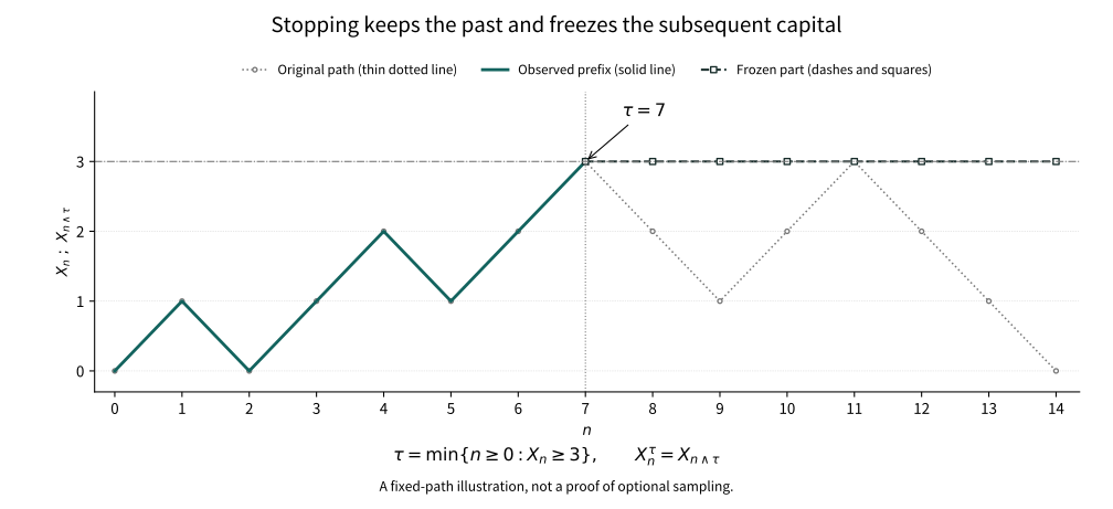
A first hit uses only the record already observed. This fixed nearest-neighbour path first reaches level 3 at step 7. The solid prefix is retained; the dashed line with square markers then stays at 3, while the thin dotted line shows the unstopped path. No randomness is sampled. This finite illustration neither proves optional sampling nor asserts expectation preservation for arbitrary stopping rules.
[Static SVG](../assets/visuals/batch16-20/stopping-prefix.en.svg) · [Vector PDF](../assets/visuals/batch16-20/stopping-prefix.en.pdf)
## 16.4 Why bounded endpoints preserve fairness
Let \(M\) be a martingale and \(S\le T\le N\) stopping times. The claim is stronger than equality of expectations:
\[
\mathbb E[M_T\mid\mathcal F_S]=M_S.
\]
For \(A\in\mathcal F_S\), expand
\[
\mathbb E[(M_T-M_S)\mathbf1_A]
=\sum_{k=1}^N\mathbb E[\mathbf1_{A\cap\{Ska)\le(1-p^a)^k.
\]
Thus \(T<\infty\) almost surely and \(E_xT<\infty\). In the fair case \(p=q=1/2\), bounded sampling at \(T\wedge n\) gives \(E_xS_{T\wedge n}=x\). The stopped positions lie between 0 and \(a\), so DCT yields
\[
P_x(S_T=a)=x/a.
\]
The horizon is random, but the capitals before and after settlement have a common deterministic bound. That bound makes passage through expectation safe.
## 16.6 The cost of waiting can also be calculated
For fair walk, \(S_n^2-n\) is a martingale: expansion of the square gives conditional cross term zero and squared increment one. Sampling at the bounded time already covered gives
\[
E_x(T\wedge n)=E_xS_{T\wedge n}^2-x^2.
\]
The left side increases to \(E_xT\); bounded convergence on the right gives \(a^2(x/a)-x^2\). Therefore
\[
E_xT=x(a-x).
\]
For \(p\ne q\), put \(r=q/p\). Since \(pr+q/r=1\), the process \(r^{S_n}\) is a martingale. Stopping inside the finite interval supplies a deterministic bound, and hence
\[
P_x(S_T=a)=\frac{1-r^x}{1-r^a}.
\]
As \(p\to1/2\) this tends to \(x/a\). Drift changes the harmonic readout: position itself suffices in the fair game, whereas an exponential removes the average drift in the biased game.
## 16.7 With only one barrier, averaging can fail
Start fair walk at 0 and let \(T\) be its first visit to 1. The finite-interval formula on \([-a,1]\) gives probability \(a/(a+1)\) of reaching 1 first. Thus \(P(T<\infty)=1\). Nevertheless,
\[
E S_{T\wedge n}=0,\qquad S_{T\wedge n}\longrightarrow S_T=1\quad\text{a.s.}
\]
The stopping rule is legitimate. What fails is uniform integrability of the finite settlements.
In fact \(ET=\infty\). If \(ET<\infty\), unit absolute increments would give
\[
|S_T-S_{T\wedge n}|\le(T-n)^+,
\]
whose expectation tends to zero. This would imply convergence in \(L^1\) and force \(ES_T=0\), contradicting \(S_T=1\). Almost sure eventual arrival and a finite average waiting cost are different assertions.
## 16.8 Where doubling stakes hide their risk
Another player stakes 1 initially, 2 after a loss, then 4, until the first win. Let \(\varepsilon_k\) be independent fair signs and \(T\) the first positive sign. The net gain is
\[
G_n=\sum_{k=1}^{n}2^{k-1}\mathbf1_{\{T\ge k\}}\varepsilon_k.
\]
At every finite horizon this is an integrable martingale with \(EG_n=0\). Before the first win the accumulated loss is \(-(2^n-1)\); once a win occurs the net gain is 1. Consequently \(T<\infty\) almost surely and \(G_T=1\), but \(G_{T\wedge n}=G_n\) is not uniformly integrable.
The uncontrolled tail can be calculated rather than merely named. The probability of no win is \(P(T>n)=2^{-n}\); on that event absolute loss is \(2^n-1\). For fixed \(K>1\), whenever \(2^n-1>K\),
\[
E[|G_n|\mathbf1_{\{|G_n|>K\}}]
=(2^n-1)2^{-n}=1-2^{-n}.
\]
However high the threshold, a later horizon leaves mean tail loss close to one. At the same time,
\[
E|G_n|=2(1-2^{-n})\le2.
\]
Even uniformly bounded absolute expectations therefore cannot secure settlement. Each finite account is integrable; its mass is concentrated on increasingly rare and increasingly expensive failure records.
Here even \(ET=2\) is finite. Integrability of the stopping time alone is therefore insufficient: the absolute-increment bound used above has disappeared. Fairness at finite horizons, integrable waiting, and an almost sure gain can coexist, paid for by unbounded stakes and uncontrolled rare losses.
## 16.9 An integrable terminal value supports unbounded settlement
Chapter 15 proved that a uniformly integrable martingale is exactly one of the form \(M_n=E[Z\mid\mathcal F_n]\) with \(Z\in L^1\). Put \(\mathcal F_\infty=\sigma(\bigcup_n\mathcal F_n)\), and use the already established limit \(M_\infty=E[Z\mid\mathcal F_\infty]\) on \(T=\infty\).
For any stopping time \(T\), split \(A\in\mathcal F_T\) into the events \(T=k\). Conditional expectation on each slice gives
\[
E[M_T\mathbf1_{A\cap\{T<\infty\}}]
=E[Z\mathbf1_{A\cap\{T<\infty\}}].
\]
Absolute integrability also needs justification: first use \(E[|M_k|\mathbf1_{A\cap\{T=k\}}]\le E[|Z|\mathbf1_{A\cap\{T=k\}}]\) and then sum. On the infinite-time slice the same identity is not automatic if the ambient \(\mathcal F\) is larger than \(\mathcal F_\infty\).
The sampling theorem itself does not require shrinking the ambient \(\mathcal F\). Instead use the canonical terminal value \(M_\infty\): Chapter 15 gives \(M_k=E[M_\infty\mid\mathcal F_k]\). Sum over the finite slices as before; on \(T=\infty\) both integrands are already \(M_\infty\), even when the event on that slice is not in \(\mathcal F_\infty\). The finite-slice absolute integrals sum to at most \(E|M_\infty|\), and the infinite slice is integrable as well. Thus \(M_T=E[M_\infty\mid\mathcal F_T]\). Taking \(Z=M_\infty\) in the first identity below and using the tower property with \(\mathcal F_S\subseteq\mathcal F_T\) yields
\[
M_T=E[Z\mid\mathcal F_T],\qquad
E[M_T\mid\mathcal F_S]=M_S\quad(S\le T).
\]
Both \(S\le T\) may be infinite, with terminal values always interpreted as \(M_\infty\). If the original arbitrary closing variable \(Z\) is retained, the first identity needs an additional condition on the infinite slice: \(\mathcal F=\mathcal F_\infty\) is sufficient, and an almost surely finite \(T\) avoids the issue. The distinction is real: let every \(\mathcal F_n\) be trivial, let \(Z\) be a hidden fair sign, and set \(T\equiv\infty\). Then \(M_T=M_\infty=0\), whereas the ambient \(\mathcal F_T=\mathcal F\) gives \(E[Z\mid\mathcal F_T]=Z\). It is the formula for an arbitrary closing variable that fails, not sampling with the canonical terminal value.
The terminal representation also explains why unbounded sampling consumes no additional tail budget. For any sub-sigma-field \(\mathcal G\), put \(V=E[M_\infty\mid\mathcal G]\). For positive \(a,K\), the event \(\{|V|>K\}\) is \(\mathcal G\)-measurable. Conditional triangle inequality, truncation and Markov's bound give
\[
\begin{aligned}
E[|V|\mathbf1_{\{|V|>K\}}]
&\le E[|M_\infty|\mathbf1_{\{|V|>K\}}]\\
&\le E[|M_\infty|\mathbf1_{\{|M_\infty|>a\}}]
+\frac{aE|M_\infty|}{K}.
\end{aligned}
\]
First make \(a\) large to control the first term, then make \(K\) large to control the second. The bound is independent of \(\mathcal G\), so all conditional averages of the same integrable terminal value form a uniformly integrable family. Taking \(\mathcal G=\mathcal F_T\) controls \(M_T\) simultaneously over all stopping times, including rules with an infinite-time slice, without finding a new dominating random variable for each rule.
## 16.10 Can one stop without uniform integrability of the entire game?
Yes. For an almost surely finite \(T\), suppose the stopped family \(\{M_{n\wedge T}:n\ge0\}\) is uniformly integrable. Chapter 15 shows convergence in \(L^1\) to \(M_T\), so \(EM_T=EM_0\). More generally, for \(S\le T\) the stopped martingale is closed; the preceding result gives \(E[M_T\mid\mathcal F_S]=M_S\). This condition concerns the rule actually used, rather than play after departure.
The stopped-family condition also permits \(T=\infty\). Put \(N_n=M_{n\wedge T}\); uniform integrability gives an integrable terminal value \(Y\) with \(N_n=E[Y\mid\mathcal F_n]\). On \(T<\infty\) the path eventually freezes, so \(Y=M_T\); on the infinite slice define settlement by \(Y\). Apply 16.9 to this stopped process: for \(S\le T\), \(E[Y\mid\mathcal F_S]=M_S\), also taking \(Y\) when \(S=\infty\). The original process need not have a terminal value everywhere.
Here \(Y\) must be chosen as the stopped process's actual almost sure and \(L^1\) limit,
\[
Y=\lim_{n\to\infty}N_n,\qquad Y\in L^1(\mathcal F_\infty),
\]
rather than another environmental variable with the same conditional averages at finite times. If \(S\) is finite and \(S\le T\), the stopped value is \(N_S=M_S\). If \(S=\infty\), then \(T=\infty\) too, and both sides are settled using this \(Y\). Uniform integrability of the stopped family thus closes the account actually frozen by the rule. On records with \(T<\infty\), the original process, if continued, may still fail to have a limit.
A convenient sufficient condition is \(ET<\infty\) together with \(|M_k-M_{k-1}|\le C\) almost surely. Then
\[
|M_{n\wedge T}|\le|M_0|+CT\in L^1,
\]
so the stopped family is uniformly integrable. In finite-interval gambling a bound on stopped position does the same job. These controls are different, but both restrict the tails in which a limit could conceal its mean.
For a nonnegative supermartingale and an almost surely finite \(T\), bounded sampling and Fatou yield only \(EM_T\le EM_0\); equality is generally unavailable. Uniform integrability of the whole supermartingale, or of the appropriate stopped family, permits the analogous limiting argument with the appropriate conditional inequality.
## 16.11 Why first visits fit the language naturally
For an adapted discrete process and a measurable state set \(B\), define \(T_B=\inf\{n\ge0:X_n\in B\}\), with the infimum of the empty set equal to infinity. Since
\[
\{T_B\le n\}=\bigcup_{k=0}^n\{X_k\in B\},
\]
this is always a stopping time; so is the first return starting at time 1. Searching for a new visit after a stopping time \(S\) remains legitimate: split according to \(S=k\le n\) and take finite unions, using only information available by \(n\).
This explains why return rules may be iterated. It does not yet say that the process starts independently afresh after each return. Stopping times make the rule legal; whether the new law depends only on present position is an additional structure.
## 16.12 What continuous paths do and do not provide
Chapter 4's particle does not appear only at integer times. The discrete theorem cannot simply stand in for continuous-time sampling, but a precise measurability fact can already be proved.
Let \(X_t\) be a continuous adapted process in a metric space and \(C\) closed. For fixed \(t\), continuity and compactness of the time interval give
\[
\{T_C\le t\}=\left\{\inf_{s\in([0,t]\cap\mathbb Q)\cup\{t\}}d(X_s,C)=0\right\}\in\mathcal F_t.
\]
Thus the first visit to a closed set is legitimate. With merely right-continuous paths, for an open set \(O\) one first has \(\{T_O
Knowing the next-step rule does not yet tell us where a long journey will lead. We now restrict to a finite or countable state space with its discrete sigma-algebra, writing the transition matrix as \(p_{ij}\). A kernel can then be drawn as a directed graph, retaining precisely the transitions with positive probability.
The probability of a finite path is the product of its edge probabilities. Thus a positive-probability route from \(i\) to \(j\) exists exactly when \(p^{(n)}_{ij}>0\) for some \(n\ge0\). Write \(i\to j\), allowing a zero-step path. Chapman–Kolmogorov makes accessibility transitive by concatenation. If both \(i\to j\) and \(j\to i\), write \(i\leftrightarrow j\). Reflexivity, symmetry and transitivity partition the states into communication classes. A chain with just one class is irreducible.
These definitions first distinguish an irreversible departure. A communication class is closed if it has no positive-probability transition out of the class: once entered, it cannot be left. Collapse each class to a vertex. The resulting graph has no directed cycle, since classes on a cycle would communicate and should have been merged. Following outward edges in a finite graph must end. Every finite chain therefore has a closed class, and every state has a route to one.
A route is not yet almost-sure entry. Finiteness supplies the missing step. Let \(B\) be the union of all closed classes and \(H=\inf\{n\ge0:X_n\in B\}\). If there are states outside, choose from each one a positive-probability path into \(B\). There are finitely many such states, so all selected path lengths are bounded by some \(L\ge1\), and all their probabilities are at least some \(\eta>0\). Arrival need not occur exactly at step \(L\); following a chosen path and entering earlier already counts.
\[
P_\mu(H>(r+1)L)\le(1-\eta)P_\mu(H>rL)
\le(1-\eta)^{r+1}.
\]
For the first inequality, condition on \(\mathcal F_{rL}\) on \(\{H>rL\}\) and use the selected path from the current state; induction gives the second. Hence \(H<\infty\) almost surely, and summing the tail gives \(E_\mu H\le L/\eta\). If every state already lies in \(B\), then \(H=0\) and no estimate is needed. Accessibility in a graph was not silently replaced by probability one: finitely many starting points supplied a uniform chance.
On an infinite space that uniform chance may disappear. Even mutual accessibility is not recurrence: a route back can exist while the chain avoids returning forever with positive probability. The return questions ahead cannot be settled merely by drawing arrows.
## 17.7 If a law settles, what can it settle to?
Do not assume that settling occurs. If the laws \(\mu P^n\) of a finite chain do converge to a probability vector \(\pi\), the next step still uses the same matrix. Passing a finite sum through the limit forces \(\pi P=\pi\). We therefore first seek a distribution preserved by one step, called an invariant distribution. This is an equation any possible limit must satisfy, not a proof that a limit exists.
Starting from an invariant distribution gives the same law to every time-shifted finite path. Indeed, the probability of \(i_0,\ldots,i_r\) is \(\pi_{i_0}\prod_{k0\) and \(p^{(n)}_{ij}>0\), then \(\pi_j=(\pi P^n)_j\ge\pi_ip^{(n)}_{ij}>0\). Any other invariant probability \(\rho\) is positive everywhere too. To prove equality, compare the ratios \(r_i=\pi_i/\rho_i\). Invariance gives
\[
r_i=\sum_j\frac{\rho_jp_{ji}}{\rho_i}\,r_j,\qquad
\sum_j\frac{\rho_jp_{ji}}{\rho_i}=1.
\]
Each ratio is a weighted average of other ratios. Finiteness ensures that a maximum is attained; equality of an average with that maximum forces every positively weighted term to attain it too. The positive weight edges reverse the original graph, whose reversal is still irreducible. The maximum propagates along reversed paths to every state. The ratio is constant, and total mass one makes the constant one. This proves uniqueness for a finite irreducible chain. The reversed weights will later acquire an interpretation through reversed time.
The proof cannot be transferred unchanged to an infinite space. For deterministic right shift \(i\mapsto i+1\) on the nonnegative integers, the averaged law from zero is uniform on the first \(N\) points. Each coordinate tends to zero, but the coordinate limit is no longer a probability. The invariant equations likewise force zero mass at zero and then at every successive point. For symmetric walk on the integer line, an invariant vector satisfies \(2\pi_j=\pi_{j-1}+\pi_{j+1}\); adjacent differences are constant, nonnegativity on all integers forces a constant sequence, and a nonzero constant is not summable. These exhibit mass leaving finite windows and an invariant measure that cannot be normalized.
## 17.8 Invariant weights may still carry a periodic clock
A chain that switches between two states at every step is irreducible and has the unique invariant distribution \((1/2,1/2)\). Yet from a fixed state its laws alternate forever between two point masses. The obstruction concerns permitted return times, not communication in space.
For a state \(i\) with a possible positive-time return, define the greatest common divisor of all its possible return lengths:
\[
d(i)=\gcd\{n\ge1:p^{(n)}_{ii}>0\}.
\]
This is its period; \(d(i)=1\) means aperiodic. The greatest common divisor retains the temporal lattice that concatenation cannot break, rather than merely the shortest possible return. If positive paths \(i\to j\) and \(j\to i\) have lengths \(a,b\), any return length \(n\) at \(j\) makes both \(a+n+b\) and \(a+b\) return lengths at \(i\). Hence \(d(i)\) divides \(n\). Interchanging states proves equality of periods throughout a communication class. The same-state comparison is immediate; for distinct states the lengths \(a,b\) can be positive.
Every state of a finite irreducible chain has a positive-time return. Fix a base \(o\), and let \(r(j)\) be the length modulo the common period \(d\) of any positive-probability path from \(o\) to \(j\), allowing the zero-step path at the base. The residue is well defined: append the same path \(j\to o\) to two choices, and their return-length difference is divisible by \(d\). Thus
\[
C_\ell=\{j:r(j)=\ell\},\qquad
p_{ij}>0\ \Longrightarrow\ r(j)=r(i)+1\pmod d.
\]
Every residue class is nonempty: traverse the first \(d\) times of a positive-probability return circuit at \(o\). Each step goes only from \(C_\ell\) to \(C_{\ell+1}\). Invariance gives these sets equal \(\pi\)-mass, hence mass \(1/d\) each. From a fixed state, however, all mass at time \(n\) lies in a single current phase. For \(d>1\), this event has probability one now and stationary probability \(1/d\), a discrepancy at least \(1-1/d\) that cannot disappear.
Waiting in place is one way to break periodicity: a positive self-loop anywhere in an irreducible class forces common period one. It is not necessary. The following three-state chain has no self-loops, but zero can return in both two and three steps:
\[
P=\begin{pmatrix}
0&1&0\\[2pt]
\tfrac12&0&\tfrac12\\[2pt]
1&0&0
\end{pmatrix},\qquad \pi=(\tfrac25,\tfrac25,\tfrac15).
\]
The graph is irreducible, and two and three have greatest common divisor one. The displayed invariant law follows directly from the incoming-flow equations and normalization. What matters is not whether every step allows a pause, but whether concatenable circuits remain constrained by a coarser common clock.
## 17.9 From no common period to routes at every sufficiently late time
Aperiodicity removes an obstruction, but we need a positive conclusion. Knowing one route between each pair of states does not make those routes equally long. To compare distributions at a common observation time, we must be able to extend different routes to a common duration.
First study returns to one state \(o\). Return lengths are closed under addition because circuits concatenate. If their greatest common divisor is one, finitely many of them, \(a_1,\ldots,a_q\), already have greatest common divisor one: as lengths are added, the gcd descends through positive integers and eventually reaches the gcd of the full set. We now prove that their nonnegative integer combinations contain every sufficiently large integer.
Work modulo \(a_1\). The residues of nonnegative combinations contain zero and are closed under addition. In a finite group such a set contains inverses too, since a positive multiple of each element is zero. It is a subgroup. Gcd one makes it the whole residue group: the least positive integer linear combination divides every \(a_j\), hence is one, so the subgroup contains one. For each residue \(\ell\), choose an actual nonnegative combination \(b_\ell\) representing it. If \(M=\max_\ell b_\ell\), any \(n\ge M\), with \(b_\ell\) congruent to \(n\), has
\[
n=b_\ell+k a_1,\qquad k\in\{0,1,2,\ldots\}.
\]
Concatenating the corresponding circuits gives positive path probability, so \(p^{(n)}_{oo}>0\) for every sufficiently large positive integer \(n\). The gcd definition has become a usable probability statement about actual paths, without concealing the arithmetic in an unnamed standard lemma.
For every pair \(i,j\), choose positive-probability paths \(i\to o\) and \(o\to j\), of lengths \(u_i,v_j\), allowing zero steps where appropriate. Finitely many states allow a single \(N\ge1\) such that \(n-u_i-v_j\) is an allowed return length whenever \(n\ge N\), for every pair \(i,j\). Chapman–Kolmogorov yields
\[
p^{(n)}_{ij}\ge
p^{(u_i)}_{io}\,p^{(n-u_i-v_j)}_{oo}\,p^{(v_j)}_{oj}>0
\qquad(n\ge N).
\]
Thus some power \(P^N\) of a finite irreducible aperiodic chain has all entries strictly positive. Conversely, if \(P^N\) is strictly positive, all states communicate, and \(P^{N+1}=PP^N\) is strictly positive because each row sums to one. Consecutive return lengths \(N,N+1\) force period one. These conditions are equivalent in the finite setting; on an infinite space positive routes for individual pairs do not supply a uniform positive lower bound.
## 17.10 How shared probability mass removes the starting point
We can now reach every state at a common time, but that alone is not yet convergence of laws. The key is that finitely many positive numbers have a common positive lower bound. Distributions arriving from different starting points then contain an identical probability component. Their remaining difference contracts after each block of the same duration.
We use the total-variation convention from Chapter 13. On a finite set \(E\),
\[
\|\mu-\nu\|_{\mathrm{TV}}
=\sup_{A\subseteq E}|\mu(A)-\nu(A)|
=\frac12\sum_{j\in E}|\mu_j-\nu_j|.
\]
The coordinates satisfying \(\mu_j-\nu_j>0\) attain the supremum; equality of total positive and negative mass explains the factor \(1/2\). This measures the largest probability discrepancy over events, rather than a chosen coordinate. For any transition matrix \(R\), the triangle inequality and row sums one give
\[
\begin{aligned}
2\|\mu R-\nu R\|_{\mathrm{TV}}
&=\sum_j\left|\sum_i(\mu_i-\nu_i)R_{ij}\right|\\
&\le\sum_i|\mu_i-\nu_i|\sum_jR_{ij}
=2\|\mu-\nu\|_{\mathrm{TV}}.
\end{aligned}
\]
Evolution cannot enlarge this discrepancy, but two-state alternation can preserve it completely. Let \(s=|E|\), take \(K=P^N\) from the preceding section, and set
\[
\delta=\min_{i,j}K_{ij}>0,\qquad
\varepsilon=s\delta\in(0,1],\qquad u_j=\frac1s.
\]
If \(\varepsilon<1\), subtract the uniform mass common to every row and normalize what remains:
\[
R_{ij}=\frac{K_{ij}-\varepsilon u_j}{1-\varepsilon},
\qquad K_{ij}=\varepsilon u_j+(1-\varepsilon)R_{ij}.
\]
The numerators are nonnegative and each row sums to \(1-\varepsilon\), so \(R\) really is a transition matrix. Multiplying any two initial laws by \(K\) makes their common \(\varepsilon u\) cancel. Nonexpansion becomes strict contraction:
\[
\|\mu K-\nu K\|_{\mathrm{TV}}
\le(1-\varepsilon)\|\mu-\nu\|_{\mathrm{TV}}.
\]
**Finite-chain convergence theorem.** If \(P\) is a finite-state irreducible aperiodic transition matrix, it has a unique invariant probability \(\pi\), and \(\mu P^n\to\pi\) in total variation for every initial law \(\mu\). More precisely, for \(0<\varepsilon<1\), the \(N,\varepsilon\) above satisfy
\[
\|\mu P^n-\pi\|_{\mathrm{TV}}
\le(1-\varepsilon)^{\lfloor n/N\rfloor}\|\mu-\pi\|_{\mathrm{TV}}.
\]
Existence, positivity and uniqueness were proved in 17.7; section 17.9 supplies \(N\); this section supplies contraction per block. Write \(n=kN+r\), \(0\le r
Two-state alternation is not absence of order; it is excessive stability demanded on the wrong clock. Even with periodicity, the averaged laws of a finite irreducible chain converge to its unique \(\pi\): every subsequential limit from 17.7 is invariant and hence identical. If the full sequence failed to converge, a subsequence bounded away from \(\pi\) would have a further convergent subsequence in the finite simplex, a contradiction. Thus for every initial \(\mu\),
\[
\frac1N\sum_{n=0}^{N-1}\mu P^n\longrightarrow\pi
\quad\text{in total variation}.
\]
Without averaging, individual phases have limits too. At common period \(d\), observing every \(d\) steps makes \(P^d\) stay within each \(C_\ell\). Its restriction is irreducible, since a positive path between states in the same phase has length divisible by \(d\). It is aperiodic because dividing all original return lengths by \(d\) leaves gcd one. Its invariant law is the normalized restriction of \(\pi\), namely \(d\pi_j\) on that class.
The normalized restriction is invariant because \(\pi P^d=\pi\) and \(P^d\) has no transitions between these classes, so its invariant equations restrict to each class. We may now apply the finite-chain theorem just proved, rather than assume a separate periodic convergence result. Starting at \(i\in C_a\), for \(0\le r
Irreducibility is not merely a label next to a theorem. Two disjoint absorbing states already give every mixture as an invariant law; no mechanism can erase which closed world the chain eventually enters. Long-term laws of a finite reducible chain must record that choice before studying stability inside each class.
Let the closed communication classes be \(D_1,\ldots,D_b\), with their unique invariant probabilities \(\pi^{(a)}\), extended by zero outside the class. Section 17.6 proved entry into their union at a finite time \(H\). The mass outside is at most \(P_\mu(H>n)\), tending to zero. For an invariant law \(\rho\), starting from \(\rho\) keeps that outside mass constant and must therefore vanish. Restricting the invariant equations to each class and using uniqueness shows that all invariant probabilities are exactly
\[
\rho=\sum_{a=1}^b c_a\pi^{(a)},\qquad
c_a\ge0,\quad\sum_a c_a=1.
\]
If every closed class is also aperiodic, the time marginals do converge, but their mixture weights depend on the initial experiment. With \(\alpha_a=P_\mu(X_H\in D_a)\),
\[
\mu P^n\longrightarrow\sum_{a=1}^b\alpha_a\pi^{(a)}
\quad\text{in total variation}.
\]
One cannot simply substitute a random entry time into a deterministic-time limit. Fix \(M\) and first restrict to \(H\le M\). Partition by \(H=h\) and \(X_H=i\). Strong Markov from 17.5 gives the subsequent law \(P^{n-h}(i,\cdot)\). Finitely many \(h\le M,i\) allow simultaneous use of within-class convergence. The actual remainder on \(H>M\) and the corresponding target mixture have the same total mass, so their total variation is at most \(P_\mu(H>M)\). Let \(n\to\infty\) first and then \(M\to\infty\) to prove the limit.
Periodic closed classes can prevent convergence at every time; retain the preceding phases or average the laws over time. The averaged version needs no aperiodicity, but still distinguishes times before and after entry. On \(H=h\le M\), \(X_H=i\in D_a\), apply strong Markov only to the terms after entry:
\[
\frac1N\sum_{n=h}^{N-1}P^{n-h}(i,\cdot)
=\frac{N-h}{N}
\left(\frac1{N-h}\sum_{k=0}^{N-h-1}P^k(i,\cdot)\right)
\longrightarrow\pi^{(a)}\qquad(N>M).
\]
There are at most \(M\) terms with \(nM\) contribute at most \(P(H>M)\) discrepancy. Let \(N\to\infty\) and then \(M\to\infty\) to obtain the same mixture \(\sum_a\alpha_a\pi^{(a)}\). No negative-time matrix power is used, and a random shift is not silently treated as deterministic. This remains a long-term statement about laws, not a sample-path ergodic theorem.
## 17.13 After stationarity, does reversed time give the same experiment?
An unchanging long-term distribution does not remove the direction of time. Reversed weights appeared in the uniqueness proof of 17.7; now read them from a stationary record. At a state with \(\pi_i>0\), the conditional probability that the preceding state was \(j\), given the current state \(i\), is
\[
\widehat p_{ij}=\frac{\pi_jp_{ji}}{\pi_i}.
\]
Invariance makes each row sum to one and gives \(\pi\widehat P=\pi\). These identities hold on countable chains as well, by summing nonnegative terms. If \(\pi_j=0\), the nonnegative terms in its invariant equation show that the positive-mass support cannot transition to \(j\). Use the formula on that support; arbitrary reversed rows at zero-mass states do not change the stationary path law.
The description extends beyond two adjacent times. For a finite path in the support, the reversed transition product telescopes:
\[
\begin{aligned}
\pi_{i_n}\prod_{k=0}^{n-1}\widehat p_{i_{k+1}i_k}
&=\pi_{i_n}\prod_{k=0}^{n-1}
\frac{\pi_{i_k}p_{i_ki_{k+1}}}{\pi_{i_{k+1}}}\\
&=\pi_{i_0}\prod_{k=0}^{n-1}p_{i_ki_{k+1}}.
\end{aligned}
\]
Thus the reversed record is Markov, but usually with the different kernel \(\widehat P\). If forward and backward records are to have the same stationary law, paths of length one force detailed balance for every pair of states:
\[
\pi_ip_{ij}=\pi_jp_{ji}.
\]
Conversely, summing detailed balance gives invariance, and multiplying along finite paths gives equal probabilities to forward and backward records. It is therefore equivalent to reversibility here. It is stronger than invariance: invariance balances total incoming and outgoing flow at each state, while detailed balance balances each pair separately.
Deterministic rotation around a directed three-cycle has invariant uniform law but no reverse edges, so it is not reversible. If each step instead waits with probability one half and moves forward with probability one half, the chain remains nonreversible but becomes finite, irreducible and aperiodic. It converges to the uniform law from every start. Conversely, deterministic two-state alternation satisfies detailed balance but fails to converge at every time because its period is two. Reversibility cannot replace aperiodicity, and convergence does not require reversibility: these notions answer different experimental questions.
## Chapter 17 Epilogue: The next-step rule and the long future
The posterior state stores the information left by successive observations; given it, the old record adds nothing to predicting the future. Markov property is therefore not a slogan about forgetting, but a test of whether the present state retains enough information. Sequential construction and stopping-time partitions give that claim an actual infinite record and preserve it after a legitimate stop.
If finding a unique invariant law had been treated as the endpoint, two-state alternation could easily have been dismissed as a minor exception. Taking it seriously separates two questions previously conflated: which law can remain invariant, and whether different initial laws approach it. The next distinction concerns permitted path durations rather than more coordinates. These distinctions exposed by counterexamples advance the question; a common positive power and common probability mass then become tools precisely suited to resolving it.
Finite space ultimately confines the chain to a closed component, making these uniform estimates possible. On an infinite lattice, arrows can still point back toward the start while a path keeps travelling away. After finding a route back, we must compute whether it will actually be taken and how many returns occur. That difference leads random walk toward visit counts and spatial dimension.
## Sources and proof scope
The unknown-bias coin, bit counterexample, cycles and finite-matrix arguments are modern mathematical reconstructions, not invented episodes from Markov's own discovery. General measurable-space existence is actually supported by [T-SEQUENTIAL](../foundations/t-sequential.md#t-sequential-extension); an original reference is Ionescu–Tulcea's 1949 [Mesures dans les espaces produits](https://cs.uwaterloo.ca/~y328yu/classics/IonescuTulcea49.pdf). Pointwise sequential-kernel data remain distinct from arbitrary finite-dimensional extension on general spaces.
The periodic arithmetic and convergence scope were checked against Cambridge's public [Markov Chains notes, sections 9.2–9.3](https://www.statslab.cam.ac.uk/~rrw1/markov/M.pdf). Here nonnegative integer combinations are proved explicitly and contraction follows from common mass in finite matrices, without a general coupling or Harris theorem. Chapter 18 develops returns and Green kernels; Chapter 42 retains general-state Harris and mixing theory. The finite results here are not counted as proofs of those general theorems.
---
# Chapter 18: Why Do Some Random Walks Return While Others Escape?
A step left and a step right leave no preferred direction on average. Yet on a three-dimensional lattice, a walker with no directional preference at any step has positive probability of never revisiting its starting point.
Chapter 4's scaling picture does not answer this question. There, many tiny steps were compressed into a finite time window. Here step size stays fixed while time extends indefinitely. We count not the final position, but how often the same place will be seen again.
## 18.1 Being able to return is not returning
For a countable-state Markov chain started at \(i\), define the first positive-time return
\[
T_i=\inf\{n\ge1:X_n=i\},\qquad f_i=P_i(T_i<\infty).
\]
The state \(i\) is recurrent if \(f_i=1\), and transient if \(f_i<1\). Starting the return rule at 1 matters: otherwise the initial visit would make the probability identically one and erase the question.
Let \(N_i=\sum_{n\ge0}\mathbf1_{\{X_n=i\}}\), counting the initial visit. The discrete strong Markov property of Chapter 17 makes the probability of another return after each return equal to \(f_i\). Induction at successive returns gives
\[
P_i(N_i\ge k)=f_i^{k-1},\qquad
E_iN_i=\sum_{k\ge1}f_i^{k-1}.
\]
A recurrent state is therefore visited infinitely often almost surely. A transient state has finitely many visits almost surely, with mean \(1/(1-f_i)\). For a general random variable infinite mean need not imply an almost surely infinite value; the geometric restart structure makes them equivalent here.
## 18.2 An infinite series records the fate of one place
Define the Green kernel
\[
G(i,j)=\sum_{n=0}^\infty p^{(n)}_{ij}=E_i\sum_{n\ge0}\mathbf1_{\{X_n=j\}}.
\]
Tonelli for nonnegative integrals gives the last equality. Consequently
\[
G(i,i)=\infty\ \Longleftrightarrow\ f_i=1,\qquad
G(i,i)=\frac1{1-f_i}\quad(f_i<1).
\]
If \(H_j\) is the first hit of \(j\), including time zero, strong Markov also gives \(G(i,j)=P_i(H_j<\infty)G(j,j)\) as a nonnegative extended integral. When the probability is zero, interpret the right side as zero, not an undefined \(0\cdot\infty\). Split over the hitting event and then accumulate future visits by monotone convergence to prove the identity.
Thus probabilities at fixed times can together answer a question about an infinite path. We use more than one marginal: the renewal relation after returns supplies the extra structure.
## 18.3 First returns split all returns into cycles
Put \(u_n=P_i(X_n=i)\) and \(a_k=P_i(T_i=k)\). Splitting according to first return gives
\[
u_0=1,\qquad u_n=\sum_{k=1}^na_ku_{n-k}\quad(n\ge1).
\]
For \(0\le z<1\) the series converge absolutely. Their generating functions satisfy \(U(z)=1+A(z)U(z)\), hence \(U(z)=1/(1-A(z))\). Letting \(z\uparrow1\) recovers the Green criterion. The first-return law may be defective: total mass below one records paths with no next cycle.
This renewal equation will begin the next chapter. For now, another readout of \(u_n\) will show how dimension changes the series.
## 18.4 How a Fourier readout selects the origin
Consider simple symmetric nearest-neighbor walk on \(\mathbb Z^d\). Each independent step chooses uniformly among \(2d\) directions. Its characteristic function is
\[
\phi(\theta)=\frac1d\sum_{j=1}^d\cos\theta_j,
\qquad\theta\in[-\pi,\pi]^d.
\]
For every integer vector \(k\), multiplying the coordinate exponential integrals yields
\[
(2\pi)^{-d}\int_{[-\pi,\pi]^d}e^{i\theta\cdot k}\,d\theta
=\mathbf1_{\{k=0\}}.
\]
Take expectation at the random position and use bounded Fubini to obtain \(u_n=(2\pi)^{-d}\int\phi(\theta)^n\,d\theta\). No general local CLT is required, and weak convergence has not been substituted for a point-probability estimate.
## 18.5 Discount infinite time before summing it
The powers \(\phi^n\) may have either sign, so summing them under an integral needs justification. First take \(0q\), the chance of hitting 0 from 1 is \(q/p\): apply Chapter 16's ruin formula on \([0,a]\) and let \(a\to\infty\). A path that hits 0 at a finite time has a finite maximum before that hit, so the union of these finite-interval events is exactly eventual hitting.
From −1 the chance of hitting 0 is one. Enlarge the left barrier in the same way, or use Chapter 12's strong law to see the position eventually tending rightward to infinity, which a nearest-neighbor path cannot do without crossing 0. Splitting on the first step gives
\[
f_0=p(q/p)+q=2q<1.
\]
For \(p0\). On recurrent records from \(i\), put \(\tau_0=0\) and let \(\tau_{r+1}\) be the first visit to \(i\) at or after \(\tau_r+\ell\). These are finite stopping times. The whole route of attempt \(r\) is revealed before the next attempt begins. If \(A_r\) denotes failure of all the first \(r\) attempts, strong Markov gives
\[
P_i(A_r)\le(1-\eta)^r.
\]
This justifies the geometric bound. Starting a possibly overlapping long attempt at every visit to \(i\) and simply multiplying success chances would not ensure conditioning at the right times. Unconditional independence of attempts is unnecessary; each attempt needs the same conditional success probability \(\eta\) given its past.
Starting from \(j\), it must also hit \(i\) almost surely. Otherwise choose a positive-probability route from \(i\) to its first arrival at \(j\), with no intervening return to \(i\), then a positive-probability future avoiding \(i\). This would give positive probability of no return to \(i\), a contradiction. Iterating strong Markov shows infinitely many visits to \(j\). Thus \(j\) and every state communicating with a recurrent state is recurrent, and recurrent classes are closed.
From any initial state, a specified transient state is visited finitely often almost surely: upon a hit, its remaining visits have the geometric law; without a hit, their number is zero. Taking a common null set over countably many states, the path eventually leaves every fixed finite set. This is a precise sense of escape, not a claim that position has a directional limit.
## 18.10 Infinitely many returns can have infinite mean spacing
A recurrent state is positive recurrent if \(E_iT_i<\infty\), and null recurrent if \(E_iT_i=\infty\). Let the mean visits to \(j\) in one complete return cycle from \(i\) be
\[
\nu_j=E_i\sum_{n=0}^{T_i-1}\mathbf1_{\{X_n=j\}},
\]
Then \(\nu_i=1\) and \(\nu P=\nu\). Shift the occupation count by one time step: times 0 through one before the return become times 1 through \(T_i\); both endpoints are \(i\), so they cancel. All interchanges are initially nonnegative integrations.
The role of stopping in the one-step shift can also be made explicit. Since \(\{n0\). Under the stationary initial law, the events “at \(i\) at time \(n\), with no later visit” are disjoint for different \(n\). Finite-block stationarity followed by a decreasing limit gives each probability \(\pi_i(1-f_i)\). Their infinite sum is at most one, forcing \(f_i=1\) for every state. No general ergodic theorem has been used.
The remainder must actually vanish. By 18.9, every state \(k\) hits \(i\) almost surely: a positive-probability hitting path with no intermediate return to \(k\) can be tried again at successive returns to \(k\), and repeated failure has a geometric bound. Put \(H_i=\inf\{n\ge0:X_n=i\}\) and \(D=E\setminus\{i\}\); let \(K=(p_{k\ell})_{k,\ell\in D}\) be the substochastic matrix killed at \(i\), and \(b=(p_{ij})_{j\in D}\). The invariant equation on \(D\) gives
\[
\pi_D=\pi_i b+\pi_DK
=\pi_i\sum_{r=0}^{N-1}bK^r+\pi_DK^N.
\]
For \(j\in D\), \(\sum_{r\ge0}(bK^r)_j=\nu_j\): these are precisely the probabilities of visits after departure from \(i\) and before its first return. The remainder has total mass
\[
\sum_{j\in D}(\pi_DK^N)_j
=\sum_{k\in D}\pi_kP_k(H_i>N)\longrightarrow0.
\]
Every hitting tail tends to zero, dominated by the summable \(\pi_k\), so dominated convergence is justified. The first term tends to \(\pi_i\nu_j\) by nonnegative monotone convergence. Include \(\nu_i=1\) and sum over all states to obtain
\[
\pi_j=\pi_i\nu_j,\qquad E_iT_i=1/\pi_i.
\]
Cycle budgets uniquely determine the invariant probability. Symmetric line walk is recurrent but, as Chapter 17 showed, has no invariant probability; it is null recurrent. Finite irreducible chains have invariant probabilities, hence positive recurrent states, though periodicity may still prevent stepwise convergence.
## 18.12 New upward records give another restart
For a real random walk \(S_n\) with independent identically distributed increments, let \(L\) be the first strict ascent above the initial value and \(H=S_L\). Their joint law may be defective: some paths never set a new high. Independent increments and stopping-time slices make the time and height increments between successive records have this same joint law.
If \(q(z,\theta)=E[z^Le^{i\theta H};L<\infty]\), with \(0\le z<1\), the sum of the joint transforms of all strict ascending records is \(\sum_{k\ge0}q(z,\theta)^k=1/(1-q(z,\theta))\). Since \(|q(z,\theta)|\le z<1\), absolute control justifies the summation. This proves the ladder renewal structure itself.
It is not yet the complete Wiener–Hopf factorization splitting the whole walk into ascending and descending parts. Strict-versus-weak boundary conventions and the full product identity still need a separate proof. This precise boundary is retained rather than declaring the entire discrete or Lévy factorization proved by naming it.
## Chapter 18 Epilogue: Revisited places divide time into cycles
Unbiased steps cross a genuine boundary between dimensions two and three. The difference is not in one jump, but in the total budget for infinitely many possible returns. The Green sum records that budget; Fourier integration turns it into competition between singularity and volume near the origin.
Whenever a return occurs, the future begins from the same state again. A record is divided into cycles. Some never finish; others finish almost surely but have infinite mean. Combining these restarts to calculate long-term waiting requires more than deciding whether a return happens: it requires understanding how cycles fill time.
## Historical sources and scope
Pólya's paper, “Über eine Aufgabe der Wahrscheinlichkeitsrechnung betreffend die Irrfahrt im Straßennetz,” appeared in volume 84 of Mathematische Annalen in 1921, pages 149–160. The discounted Fourier argument here is a modern reconstruction using our established characteristic functions and integration tools, not a claim to reproduce his original proof. See the [original publication record](https://doi.org/10.1007/BF01458701). The complete classification here concerns simple symmetric nearest-neighbor lattice walk; arbitrary jumps, dependent steps or general groups require proofs beyond a slogan about dimension.
---
# Chapter 19: Waiting for a New Beginning
Each return to the origin starts another wait. If return restores the same future, a long record can be read in cycles between returns rather than in single steps.
Yet a cycle encountered at an arbitrary roadside observation time is not a cycle chosen uniformly by its arrival index. Short cycles pass quickly; long ones occupy more time. An observer with no predictive knowledge is consequently more likely to land in a longer wait.
Counting cycles by arrivals and locating oneself by elapsed time assign different probabilities to the same random intervals.
## 19.1 Rebuilding a clock from waiting intervals
Let \(X_1,X_2,\ldots\) be independent identically distributed strictly positive real variables with law \(F\). Put
\[
S_0=0,\qquad S_n=X_1+\cdots+X_n,\qquad
N(t)=\max\{n:S_n\le t\}.
\]
The \(S_n\) are renewal times, and \(N(t)\) counts renewals by \(t\), excluding the initial point. Strict positivity prevents infinitely many zero-length cycles at one instant. Even with infinite mean, \(S_n\to\infty\) almost surely: choose \(\delta>0\) with \(p=P(X_1\ge\delta)>0\); the independent Bernoulli strong law supplies infinitely many such intervals. Thus the count is finite for each finite \(t\).
The model assumes independent cycles. Successive returns to a recurrent Markov state provide such cycles after the initial return. A transient state's missing return mass must be handled separately, not treated as a finite waiting interval.
## 19.2 Finite-time counts need a mean budget too
Define the renewal measure
\[
U(B)=\sum_{n\ge0}P(S_n\in B),\qquad U([0,t])=1+EN(t).
\]
Choose the preceding \(\delta,p\). If \(S_n\le h\), at most \(\lfloor h/\delta\rfloor\) among the first \(n\) intervals can be successes of length at least \(\delta\). The trial count needed for the next success is a sum of finitely many geometric waits of mean \(1/p\). Hence
\[
U([0,h])\le\frac{\lfloor h/\delta\rfloor+1}{p}<\infty.
\]
More importantly, for every \(t\ge0\), \(U([t,t+h])\le U([0,h])\). Consider the first renewal entering \([t,\infty)\). If it overshoots the interval there are no points inside; otherwise the remaining count is no larger than the count in a fresh renewal process over length \(h\). Split by the index of first entry and use independence of subsequent intervals to prove the expectation bound. Denote the common bound by \(C_h\). It will control every tail passage for which pointwise convergence alone is inadequate.
## 19.3 The strong law first supplies the average pace
Write \(\mu=EX_1\in(0,\infty]\). With finite mean, the strong law and \(S_{N(t)}\le t0\) is the largest number with \(P(X_1\in d\mathbb Z)=1\); otherwise it is nonarithmetic. This is an additive group through zero, not Chapter 13's affine lattice span for a fixed number of summands. Support \(\{1,3\}\) has renewal span 1 despite parity restrictions at fixed sample size. The discrete waiting law on \(\{1,\sqrt2\}\) is nonarithmetic.
Infinite addition does not automatically erase this distinction. With every interval equal to 1, observation phase persists forever. The nonarithmetic proof must exclude hidden periodicity rather than confusing lack of density with presence of a period.
## 19.6 Why a permutation zero–one lemma is needed
A renewal depends on the sum of the intervals accumulated so far. Permuting finitely many intervals changes early arrival order, but not sufficiently late partial sums. This concrete symmetry fits our problem better than saying that distant variables are independent of the past: the limit under study may still use every interval and need not be an obvious tail event.
The required zero–one law turns invariance under finite rearrangement into determinism. It does not make every symmetric statistic constant; a finite sample sum is certainly random. The decisive condition is that a readout of an infinite record be unchanged by every finite permutation.
We first prove the special tool required. For an iid sequence, an event \(A\) invariant under every finite coordinate permutation has probability \(P(A)\) equal to zero or one. Chapter 15's upward conditional-expectation theorem approximates \(\mathbf1_A\) in \(L^1\) by finite-prefix conditional averages. Threshold at one half to obtain an event \(B\) in the first \(m\) coordinates with \(P(A\triangle B)<\varepsilon\).
The finite approximation deserves to be explicit. Put \(\mathcal H_m=\sigma(X_1,\ldots,X_m)\) and \(D_m=E[\mathbf1_A\mid\mathcal H_m]\). Upward convergence gives \(E|D_m-\mathbf1_A|\to0\). For \(B=\{D_m>1/2\}\),
\[
P(A\triangle B)\le 2E|D_m-\mathbf1_A|.
\]
At every misclassified point the conditional average differs from the true indicator by at least one half. Finite-prefix approximation does not assume that the whole event depends on finitely many coordinates; it makes the probability of an incorrect decision arbitrarily small.
For any finite-prefix event \(C\), use a finite permutation moving all coordinates of \(B\) beyond those of \(C\). The resulting \(B'\) is independent of \(C\), and iid symmetry together with invariance of \(A\) still gives \(P(A\triangle B')<\varepsilon\). Therefore
\[
|P(A\cap C)-P(A)P(C)|\le2\varepsilon.
\]
Let epsilon vanish, then extend \(C\) to the full sequence sigma-field by pi–lambda. The event \(A\) is independent of itself. Applied to all rational level sets of a bounded permutation-invariant variable, this makes the variable almost surely constant. This proves the needed Hewitt–Savage-type lemma without importing later exchangeability or ergodic theory.
## 19.7 A bounded harmonic readout cannot retain nonarithmetic oscillation
Let bounded continuous \(h\) satisfy \(h(t)=\int h(t-x)F(dx)\). For fixed \(t\), the variables \(h(t-S_n)\) form a bounded martingale, with an almost sure and \(L^1\) limit. A finite permutation eventually leaves partial sums unchanged, hence leaves that limit unchanged. The preceding lemma makes the limit constant, with mean \(h(t)\). The closed-martingale identity then forces \(h(t-X_1)=h(t)\) almost surely.
The strongest step sends the random limit back to finite time. Define \(H_t=\limsup_n h(t-S_n)\) on every record. A finite permutation eventually leaves partial sums unchanged, so this variable really has the invariance required above. Martingale convergence also identifies it with the actual limit. Hence \(H_t=h(t)\) almost surely, and boundedness gives
\[
h(t-S_n)=E[H_t\mid\mathcal H_n]=h(t).
\]
Taking \(n=1\) gives exact invariance under a random step. We have not guessed invariance under each step from invariance on average: the zero–one law and the closed-martingale identity bridge precisely that gap.
Continuity extends the identity to every step in the support, for each \(t\). Thus \(h\) is invariant under the additive group generated by the support. A subgroup of the line that is not a discrete \(d\mathbb Z\) contains arbitrarily small positive elements; integer multiples approximate any real number, so the group is dense. Nonarithmeticity and continuity force \(h\) to be constant.
Extending an almost-sure step identity to the support also has a deterministic reason. For fixed \(t\), the \(x\) satisfying \(h(t-x)=h(t)\) form a closed set of full \(F\)-measure, hence contain the support of \(F\). This works for every \(t\) separately and yields a function identity at all translated positions. Replacing \(t\) by \(t+x\) gives invariance in the reverse direction too.
Why are a grid and a dense group the only alternatives? Let \(G\) be the group generated by the support. If the infimum \(d\) of its positive elements is positive, differences of elements approaching that infimum eventually have absolute value below \(d\), so must vanish. Thus \(d\in G\); division with remainder makes every group element a multiple of \(d\), giving \(G=d\mathbb Z\). If the infimum is zero, integer multiples of arbitrarily small positive elements approximate any real number. Nonarithmeticity therefore removes exactly the periods that a nonconstant continuous harmonic readout could retain.
For a bounded function on the integers and positive integer increments, the same martingale proof applies. If the support has greatest common divisor one, it generates the entire integer group, and the function is constant there. This harmonic mechanism explains how the local renewal limit removes periodic oscillation.
## 19.8 Finding the constant on a lattice first
Rescale arithmetic span to 1. Put \(u_n=U(\{n\})\), zero at negative indices. Strictly positive integer intervals allow at most one renewal at any point of a path, so \(0\le u_n\le1\). The renewal recursion is \(u_n=\mathbf1_{\{n=0\}}+\sum_{k\ge1}p_ku_{n-k}\).
From any integer sequence tending to infinity, extract a subsequence simultaneously for every fixed integer offset so that \(u_{n_j+\ell}\to v(\ell)\). Domination by 1 passes the recursion through the sum, giving \(v(\ell)=\sum_kp_kv(\ell-k)\). The integer harmonic lemma makes \(v\equiv c\).
Exactly one renewal cycle contains each time, yielding the identity
\[
1=\sum_{k=0}^nP(X_1>k)u_{n-k}.
\]
With finite mean, the tail weights sum to \(\mu\). Truncation followed by the bound 1 controls the remainder, giving \(1=c\mu\). Every subsequence has this same limit, hence \(u_n\to1/\mu\). Restoring span gives \(d/\mu\). We have identified mass at individual allowable renewal points, rather than only an averaged cycle rate.
## 19.9 Without a grid, select a local limit
Moving a window far out is not renormalizing a probability. The renewal measure usually has infinite mass on the whole line, so probability tightness and prevention of mass escape cannot simply be invoked. We only require a common budget in every fixed-length window. That permits local subsequential convergence, while still allowing the candidate limit to be zero.
The selection tool is exactly the real-line result already proved in T-STIELTJES: uniform mass bounds on each compact interval give one subsequence converging for every continuous compactly supported test function simultaneously. Choosing unrelated subsequences for different tests would leave the renewal equation without a common limiting measure.
The nonarithmetic conclusions here through 19.11 assume strictly positive iid intervals, a nonarithmetic law and \(0<\mu<\infty\); the arithmetic case separately retains its phase. Extend \(U\) by zero on the negative half-line. For any \(t_j\to\infty\), write \(U_t(B)=U(t+B)\). The uniform local bound in 19.2 gives a subsequence of these translated measures converging against continuous compactly supported test functions to a locally finite measure \(\lambda\). [T-STIELTJES](../foundations/t-stieltjes.md#t-stieltjes-selection) proves this selection through rational diagonal extraction, monotone functions and a pushforward of level-axis length.
Write \(U_t(g)=\int g(y)U_t(dy)\). The translated renewal equation is \(U_t(g)=g(-t)+\int U_t(g(\,\cdot+x))F(dx)\), fixing the direction of translation. If the support of \(g\) lies in an interval of length \(H\), every inner absolute integral is at most \(\|g\|_\infty C_H\), uniformly in \(x,t\). For each fixed \(x\) the translated test function is still continuous and compactly supported. Pass to the subsequential limit and then use this common bound under the probability \(F\), together with \(g(-t_j)\to0\), to obtain \(\lambda=F*\lambda\). More explicitly, for any continuous compactly supported \(g\), the function
\[
h(t)=\int g(t-y)\lambda(dy)
\]
is bounded and continuous and satisfies the harmonic equation of 19.7. The uniform interval bound gives boundedness; uniform continuity of \(g\) and the mass bound on a slightly enlarged support give continuity. Thus \(h\) is constant.
The limit measure inherits a slightly enlarged uniform window budget. Cover any interval of length \(H\) by a continuous piecewise linear function supported on an interval wider by only 2. Passing its integrals to the subsequential limit bounds the interval's \(\lambda\)-mass by \(C_{H+2}\). Continuity of the smoothed readout can consequently be quantified: for \(|r|\le1\),
\[
|h(t+r)-h(t)|\le C_{H+4}\,\omega_g(|r|),
\]
where \(\omega_g\) is the uniform continuity modulus of \(g\) extended over the line. The bound is independent of \(t\) and vanishes as \(r\to0\). The same window budget bounds absolute integrals before Fubini interchanges the convolutions, giving \(h(t)=\int h(t-x)F(dx)\). Every hypothesis of the harmonic lemma thus comes from local mass control, not from an unproved density.
It follows that \(\lambda\) is translation invariant: every test function has equal integrals under every translate. Approximate intervals from inside and outside by continuous piecewise linear functions to obtain equality of translated interval masses. Point masses must vanish, since arbitrarily many distinct translates of an atom would violate local finiteness. Interval mass therefore depends only on length, is additive and monotone in length. Establish linearity for rational lengths, then squeeze real lengths between rationals. Consequently \(\lambda=c\,dx\).
## 19.10 The normalization cannot be guessed
It remains to find \(c\). Each path's renewal intervals partition the time axis, so for \(t\ge0\),
\[
1=\int_{[0,t]}\overline F(t-s)U(ds),\qquad \overline F(x)=P(X_1>x).
\]
Translate along the selected \(t_j\). On a fixed window \([-A,0]\), the integrand is bounded and monotone, with at most countably many jumps. The limit measure \(c\,dx\) gives them no mass, so Riemann step approximation allows passage to the limit.
This identity observes an unfinished cycle: after a renewal at \(s\), the probability of no further renewal by \(t\) is \(\overline F(t-s)\). Distinct renewal indices describe disjoint last-renewal events, and their sum is exactly one. Unlike an asymptotic mean count, this is an exact budget valid at each time.
Fix \(A\) and take the selected \(t_j>A\). In coordinates \(y=s-t_j\), the integrand inside the window is \(\mathbf1_{[-A,0]}(y)\overline F(-y)\). It is bounded and Riemann integrable; T-STIELTJES handles its endpoints when passing to the candidate \(c\,dy\). The remaining task is to ensure that no mean mass has been lost outside the window.
Outside that window, merely writing DCT would be insufficient. For fixed mesh \(h>0\), the uniform local bound controls the tail by
\[
C_h\sum_{k\ge\lfloor A/h\rfloor-1}\overline F(kh).
\]
More explicitly, take \(A\ge3h\) and put \(K=\lfloor A/h\rfloor-1\). The tail function is decreasing, hence
\[
\sum_{k\ge K}\overline F(kh)\le\frac1h\int_{(K-1)h}^{\infty}\overline F(u)\,du\longrightarrow0
\quad(A\to\infty).
\]
The mesh \(h\) is fixed before \(A\) grows; no uncontrolled \(C_h/h\) is allowed to vary along with the mesh. First let \(j\to\infty\) inside the fixed window. The difference between budget one and \(c\int_0^A\overline F\) is bounded by this common tail bound. Only then let \(A\to\infty\). Finite mean enters not to select a local limit, but to carry the infinite cycle budget through that limit.
Finite mean makes the decreasing tail function integrable, so this fixed-mesh tail sum vanishes. Therefore \(1=c\int_0^\infty\overline F(x)dx=c\mu\). All subsequential candidates coincide, proving the full local renewal limit
\[
U((t,t+h])\longrightarrow h/\mu\qquad(h>0).
\]
A unique subsequential candidate must still yield convergence at all times. If the integral of some continuous compactly supported test failed to approach the identified value, there would be times tending to infinity whose integrals stay at least a fixed positive distance away. Local selection would extract a subsequence, but the preceding argument would again force its limit to be \(dx/\mu\), a contradiction. For window indicators, the Riemann bounds and vanishing endpoint atoms in T-STIELTJES then give the interval limit above.
This explains why we studied arbitrary local candidates instead of guessing a density from the elementary theorem. Uniqueness of local shape removes oscillation; the global budget identifies the constant. They solve different difficulties.
This covers every strictly positive nonarithmetic waiting law with finite mean, without density, second-moment or spread-out assumptions. No unproved ergodic theorem has entered.
## 19.11 What integrability does the key renewal theorem need?
Take a Borel measurable real function \(g\), so its integral against a possibly singular renewal measure is actually defined. Direct Riemann integrability controls actual point values, not merely a Lebesgue almost-everywhere equivalence class.
Extend \(g\) by zero on negative arguments. It is directly Riemann integrable if its positive and negative parts have mesh upper and lower sums converging to the same finite values as the mesh vanishes, and its absolute-value upper sum is finite for a sufficiently fine fixed mesh. This controls both local oscillation and distant spikes. Mere Lebesgue integrability does not control sampling by the renewal measure at particular time points.
For a nonnegative function let \(I_k(h)=[kh,(k+1)h)\), \(a_k(h)=\sup_{I_k(h)}g\) and \(b_k(h)=\inf_{I_k(h)}g\). The mesh sums are
\[
\overline R_h(g)=h\sum_{k\ge0}a_k(h),\qquad
\underline R_h(g)=h\sum_{k\ge0}b_k(h).
\]
They must tend to the same finite value as \(h\downarrow0\). For signed functions treat positive and negative parts separately, retaining a finite absolute upper sum on a fixed mesh. Compared with a finite integral, this supplies an additional visible budget: every cell must account for its largest value that the renewal measure might hit.
A nonnegative decreasing integrable function with finite initial value is an example: upper and lower sums differ by at most \(h g(0)\), and the upper sum is at most \(h g(0)+\int_0^\infty g\). Finitely many jumps do not change the conclusion. This includes the truncated tail functions that will arise from age and residual life; the test class is dictated by the problem.
Writing the full tail estimate reveals its role. Fix a mesh \(h\) with finite absolute upper sum, and let \(a_k^{*}(h)=\sup_{I_k(h)}|g|\). At every observation time,
\[
\int_{\substack{0\le s\le t\\t-s\ge A}}|g(t-s)|\,U(ds)
\le C_h\sum_{k\ge\lfloor A/h\rfloor}a_k^{*}(h)\longrightarrow0
\quad(A\to\infty).
\]
Each term uses just one reflected window of length \(h\); any part lying on the negative half-line has zero renewal mass. The right side is the tail of an already summable fixed sequence, entirely independent of \(t\). Inside a finite window, DRI also gives ordinary Riemann integrability, allowing the local limit to apply. Only after combining the two parts is the limit of the entire convolution justified.
For compactly supported Riemann-integrable functions, the interval limit of 19.10 and step bounds first give the convolution limit. For general \(g\), the fixed-mesh far convolution tail is bounded by \(C_h\) times the corresponding upper-envelope tail sum; it vanishes as the truncation bound \(A\to\infty\), uniformly over observation times \(t\ge0\). Truncate, take the long-time limit, then enlarge the truncation. This proves the nonarithmetic key renewal theorem:
\[
\int_{[0,t]}g(t-s)U(ds)\longrightarrow\frac1\mu\int_0^\infty g(s)ds.
\]
For arithmetic span \(d\), a sum cannot be replaced by an integral. At fixed phase \(r\in[0,d)\), if the sampled sequence is absolutely summable, 19.8 and the bound \(u_n\le1\) give
\[
(U*g)(nd+r)\longrightarrow\frac d\mu\sum_{k\ge0}g(kd+r).
\]
The arithmetic formula can also be checked directly. Along \(t=nd+r\), expand the convolution as \(\sum_{k=0}^n u_{n-k}g(kd+r)\), where \(u_j=U(\{jd\})\). For fixed \(k\), the coefficient tends to \(d/\mu\) and never exceeds one; the absolutely summable sampled sequence supplies domination. DRI ensures that summability: choose mesh \(ha,R_t>b\) as the integral of \(\overline F(t+b-s)\) over \(sa\}}\overline F(u+b)\) is piecewise monotone and integrable, hence directly Riemann integrable.
The last renewal index is not an independently chosen index. Fix \(n\) first, observe \(S_n\), and use independence of the next interval from that prefix. Nonnegative summation permits Tonelli and gives exactly
\[
P(A_t>a,R_t>b)
=\int_{[0,t]}\mathbf1_{\{t-s>a\}}\overline F(t+b-s)\,U(ds).
\]
The strict inequality also retains the convention for observations exactly at renewal epochs. The forcing function has one upward jump at \(a\) and decreases thereafter; finite mean controls its tail integral. The conditions of 19.11 have therefore been checked individually, rather than inferred from resemblance to a density.
In the nonarithmetic finite-mean case, the key renewal theorem gives
\[
P(A_t>a,R_t>b)\longrightarrow
\frac1\mu\int_{a+b}^\infty\overline F(u)du
=\frac{E(X_1-a-b)^+}{\mu}.
\]
This comes from an exact last-cycle decomposition rather than inserting an independent sample at a random time. In the arithmetic case use the phase-dependent sum of 19.11. If every cycle has length 1, age is the observation time's fractional part and residual life is fixed by the same phase.
## 19.14 Why longer intervals are easier to encounter
Construct the limiting joint law by first taking length-biased \(L\), with \(P(L\in dx)=xF(dx)/\mu\), then independent \(V\sim\mathrm{Unif}(0,1)\), and setting age to \(VL\), residual to \((1-V)L\). Given the length, positions satisfying both inequalities occupy length \((L-a-b)^+\). Integration under the length-biased law recovers 19.13.
Length bias is visible along an actual record as well as identifiable by a formula. For any bounded Borel function \(\psi\), a complete interval of length \(X_k\) contributes readout \(X_k\psi(X_k)\). The reward theorem of 19.12 and control of the unfinished interval give
\[
\frac1T\int_0^T\psi\bigl(X_{N(s)+1}\bigr)\,ds
\longrightarrow\frac{E[X_1\psi(X_1)]}{\mu}\quad\text{a.s.}
\]
Uniformly choosing an observation time in an increasingly long record therefore produces the length-biased law. This time-average statement does not even require nonarithmeticity. Unlike a fixed late-time distribution, uniform time observation averages over the grid phase as well.
Given encountered length \(\ell\), the fraction of interior positions with age and residual exceeding \(a,b\) is \((\ell-a-b)^+/\ell\). Multiplying by \(\ell F(d\ell)/\mu\) cancels the denominator and gives the preceding tail integral. The late-time law from the renewal theorem and the time weights from cycle rewards thus express the same geometry.
This is the inspection paradox: the observer learns no hidden fact, but longer intervals occupy more time. The deterministic sample in the figure displays this weighting without replacing the infinite renewal proof.
With finite second moment, the encountered whole interval has mean \(EX_1^2/\mu\); age and residual each have mean \(EX_1^2/(2\mu)\). With infinite second moment these remain extended nonnegative integral identities. It would be wrong to conclude that residual life always exceeds the mean ordinary whole interval: for a constant interval it is half that length. What is necessarily length-biased is the entire interval encountered by the observer.
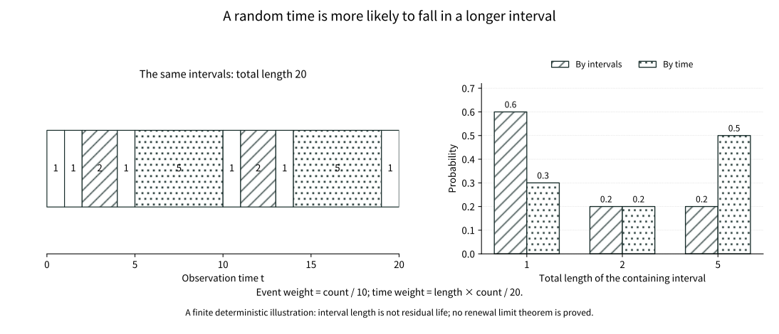
The same ten intervals produce different length distributions under uniform interval sampling and uniform time observation. Lengths 1, 2 and 5 occur 6, 2 and 2 times: their event weights are 0.6, 0.2 and 0.2, but their time weights are 0.3, 0.2 and 0.5. Longer intervals occupy more time, raising the mean containing-interval length from 2 to 3.2. This deterministic illustration on a total length of 20 is not a proof of stationary renewal construction or a renewal limit theorem. Containing-interval length is not residual life.
[Static SVG](../assets/visuals/batch16-20/inspection-length-bias.en.svg) · [Vector PDF](../assets/visuals/batch16-20/inspection-length-bias.en.pdf)
## 19.15 Making the whole renewal record stationary
Take bilateral iid intervals and root a renewal point at zero, obtaining a locally finite configuration \(\Phi\) on both sides. Use only the sigma-field generated by counts in bounded intervals, without assuming general point-process or Palm theory. Let \(\theta_s\) move the observation origin to \(s\). Length-bias the central interval, place the origin uniformly inside it, and append independent ordinary intervals in both directions. This constructs a probability \(Q\) satisfying, for every bounded measurable configuration function \(H\),
\[
QH=\frac1\mu E\int_0^{X_1}H(\theta_s\Phi)ds.
\]
Both the probability and measurability of this construction can be made explicit without general point-process theory. For the point-rooted record, take bilateral iid intervals \((X_k)_{k\in\mathbb Z}\), use 19.1 on the positive side, and define \(S_{-n}=-\sum_{j=0}^{n-1}X_{-j}\) for \(n\ge1\) on the negative side. Take an independent length-biased central interval \(L\) and uniform variable \(V\), place its ends at \(-VL\) and \((1-V)L\), and append ordinary iid intervals on both sides. The two outward partial sums diverge, so bounded windows contain finitely many points. Conditional on central length, the uniform-position factor \(1/L\) cancels the size-bias factor \(L/\mu\), yielding the cycle-integral formula above. Taking \(H=1\) checks total mass one.
For a bounded Borel interval \(B\), the translated count is \(\sum_{k\in\mathbb Z}\mathbf1_{\{S_k-s\in B\}}\), jointly measurable in the interval sequence and \(s\). Counts generate the configuration sigma-field; a function monotone-class argument then makes general bounded measurable \(H(\theta_s\Phi)\) jointly measurable too. Moving the observation origin randomly is an actual measurable experiment, not a formal symbol.
This gives more than an age-residual pair: it makes the entire configuration stationary. For \(t>0\), the exact difference of translated integration intervals is
\[
\mu\{Q(H\circ\theta_t)-QH\}
=E\int_{X_1}^{X_1+t}H(\theta_u\Phi)du
-E\int_0^tH(\theta_u\Phi)du=0.
\]
The stationarity proof uses the same bilateral iid record after rerooting; it does not assume independence between central length and the entire rerooted record. With \(u=X_1+v\), the first expected integral becomes \(E\int_0^tH(\theta_v(\theta_{X_1}\Phi))\,dv\). Rerooting merely shifts every interval index by one, so \(\theta_{X_1}\Phi\) has the original point-rooted law. Fixed length \(t\) and boundedness permit Fubini, making the two terms cancel exactly. A law rooted at an arrival has been converted into a stationary law observed in time; these are different initial laws.
Moving the point root from 0 to the next renewal at \(X_1\) merely reindexes the bilateral iid intervals, preserving their joint law. Both final integrals have fixed length \(t\), so boundedness ensures integrability. Negative shifts follow by inverse composition. This proves stationarity rather than guessing a stationary residual density. With arithmetic intervals, stationarity under all real shifts also randomizes the grid phase through the uniform interior location; fixed-grid observations retain their discrete phase version.
## 19.16 Which wish fails when the mean is infinite?
If \(P(X_1>x)=(1+x)^{-\alpha}\), \(0<\alpha<1\), every interval is still finite and renewals occur indefinitely, but \(EN(t)/t\to0\) and \(N(t)/t\to0\) almost surely. There is no probability obtained by normalizing \(xF(dx)\) with a finite \(\mu\); age and residual cannot use 19.13's finite-mean equilibrium formula.
Local limits and equilibrium probabilities must be separated here. Local selection and harmonic identification do not require finite mean; even when \(\mu=\infty\), a candidate is \(c\,dx\). Using only the fixed-window inequality from the cycle budget gives \(1\ge c\int_0^A\overline F(u)\,du\) for every \(A\). Hence \(c=0\), and nonarithmetic fixed-length window masses tend to zero. In the arithmetic case, retaining finitely many terms of the tail-sum identity in 19.8 likewise forces every subsequential constant to be zero.
This does not produce a zero probability law for age and residual life. Mass in finite windows can disappear into increasingly long cycles. The tail function required for the age problem now has infinite integral and fails the DRI hypothesis of the key theorem; \(xF(dx)\) cannot be normalized either. Infinite mean still allows a provable local zero limit, but removes the budget that made a typical observation cycle into a probability law.
Cycles still fill the time axis, but a finite mean cycle no longer supplies a normalizing budget. This does not say every infinite-mean limit is impossible. It identifies exactly why the stationary length bias and finite-mean limits in this chapter need their hypotheses.
## Chapter 19 Epilogue: An arrival and a time have different weights
Sampling by arrivals counts every cycle once. Sampling by time gives every cycle weight proportional to length. The same random record therefore admits two different notions of a typical observation.
The strong law gives the average pace, the local renewal limit stabilizes short windows, and length bias explains the observer's longer interval. All depend on restart structure, but each needs its own tail, periodicity and integrability assumptions.
So far restarts form a line: one cycle ends and the next follows. If one ending produces several new individuals, each beginning the same experiment independently, the line branches into a family.
## Historical sources and scope
Blackwell's 1948 [A renewal theorem](https://doi.org/10.1215/S0012-7094-48-01517-8) and 1953 [Extension of a renewal theorem](https://msp.org/pjm/1953/3-2/pjm-v3-n2-p03-p.pdf) are original sources for local renewal theory. Smith's 1958 survey [Renewal Theory and its Ramifications](https://doi.org/10.1111/j.2517-6161.1958.tb00294.x) discusses renewal and regenerative applications. The harmonic, permutation and cycle-integral proofs here are modern reconstructions for strictly positive iid cycles. They do not establish renewal theory for general signed increments, an ergodic theorem or Palm duality.
---
# Chapter 20: How Does One Ancestor Become a Random Family?
Record a family's population generation by generation. Its mean is the easiest quantity to calculate: if individuals reproduce independently with mean offspring \(m\), one ancestor has \(m^n\) descendants on average in generation \(n\). When \(m>1\), that mean follows an increasing exponential curve.
An extinct tree certainly cannot follow that curve. Yet even among families that survive forever, the mean need not supply the right scale. A family can continue indefinitely while its population divided by \(m^n\) tends to zero. The issue is no longer just why some families die out, but why an average can overstate the growth of almost every surviving tree.
A more accurate calculation of mean population cannot resolve the distinction. We must discover whether the mean comes from many families of ordinary size or from increasingly rare, increasingly enormous ones. Observing trees with weight proportional to their descendants will turn the latter contributions from elusive exceptions into phenomena that can be studied directly under another probability law.
## 20.1 Let an actual family tree grow
First specify the family. An offspring count \(L\) is a nonnegative integer with \(p_k=P(L=k)\). Every born individual independently uses this same reproduction rule. The count is always finite; its mean is a separate question, not a prescribed population multiplier.
Label potential individuals by finite words of positive integers: the empty word is the ancestor, and \(uj\) is child \(j\) of individual \(u\). This label set is countable. Assign independent counts \(L_u\) to every word, then retain the ancestor and recursively the children with \(j\le L_u\). Experiments assigned to unborn words do not become observations of the actual family. Chapter 8's countable product space supports the construction.
Write \(Z_n\) for the number of actual individuals in generation \(n\). Every generation is finite: starting from one ancestor, finitely many individuals each have finitely many children. Listing reproduction experiments within each generation gives
\[
Z_0=1,\qquad Z_{n+1}=\sum_{j=1}^{Z_n}L_{n,j}.
\]
This is the single-type Galton–Watson process. Let \(\mathcal F_n\) reveal the actual tree through generation \(n\): it specifies who is present, but not those individuals' offspring counts. Given \(\mathcal F_n\), the reproduction experiments on the right remain independent with the original offspring law. Revealing their results prematurely would change the conditional averages used below.
The nineteenth-century disappearance of surnames provides one historical entrance to this model. Watson and Galton's paper published in 1875 studied how many representatives of a paternal surname remain after several generations, explicitly simplifying matters through nonoverlapping generations. We retain that real question, but our individuals are abstract reproduction units. Independence, identical laws and separate generations are stated assumptions, not facts about population history, and later martingale arguments must not be attributed retrospectively to the early authors.
## 20.2 Why extinction selects the smallest root
With many independent families in one generation, enumerating every possible composition of the next generation quickly becomes unwieldy. The offspring generating function collects those combinations into a single readout:
\[
f(s)=E[s^L]=\sum_{k=0}^{\infty}p_ks^k,\qquad 0\le s\le1,\qquad 0^0=1.
\]
Given the current tree, offspring counts are independent, so \(E[s^{Z_{n+1}}\mid\mathcal F_n]=f(s)^{Z_n}\). Writing \(f_n(s)=E[s^{Z_n}]\), we obtain \(f_{n+1}=f_n\circ f\) with \(f_0(s)=s\), hence \(f_n=f^{\circ n}\). Different families within a generation require multiplication; successive generations require composition. The two operations record different independence structures.
Set \(s=0\) and write \(q_n=P(Z_n=0)=f^{\circ n}(0)\). Zero population cannot recover, so these extinction events increase and \(q_n\uparrow q\), with \(q\) the probability of eventual extinction. Bounded convergence makes \(f\) continuous on \([0,1]\), giving \(q=f(q)\). The equation alone is insufficient, since 1 is always a root.
If \(a\in[0,1]\) satisfies \(f(a)=a\), iteration of the increasing function \(f\), starting with \(0\le a\), gives \(q_n\le a\) for every \(n\). Therefore
\[
q=\min\{s\in[0,1]:f(s)=s\}.
\]
Minimality comes from the increasing limit of finite-generation events, not an arbitrary choice after solving an equation. Starting from \(r\) ancestors, independent subtrees give population generating function \((f^{\circ n}(s))^r\) and extinction probability \(q^r\). Any finite initial family can now be treated without enumerating its whole genealogy afresh.
## 20.3 The mean separates regimes, not individual futures
Assume henceforth a finite mean \(m=EL\). If \(m=0\), offspring is zero almost surely and extinction occurs in the next generation. Otherwise monotone convergence of the nonnegative series gives \(f'(1-)=m\). Convexity of the generating function links the mean to its fixed-point geometry.
When \(m<1\), we have \(f'(s)\le m<1\) for \(00\) and some \(p_k>0\) with \(k\ge2\). Strict convexity places the graph above its tangent \(s\mapsto s\) at 1, giving \(f(s)>s\) for \(s<1\). Both families become extinct almost surely.
If \(L\equiv1\), exactly one individual persists in every generation: this critical exception must be separated. When \(m>1\), the left derivative makes \(f(s)-s<0\) for \(s<1\) sufficiently close to 1, while its value at 0 is nonnegative. Continuity gives a root \(q<1\), and strict convexity allows only the roots \(q,1\). If \(p_0=0\), the smaller root is 0; if \(p_0>0\), then \(0
Given the tree already grown, next-generation mean population is \(mZ_n\), hence \(EZ_n=m^n\). For \(m>0\), divide out this predictable growth and put
\[
W_n=\frac{Z_n}{m^n},\qquad
E[W_{n+1}\mid\mathcal F_n]=W_n,\qquad EW_n=1.
\]
This is a nonnegative martingale, not an independent sequence: one ancestor's descendants influence many subsequent generations together. Chapter 15 gives \(W_n\to W<\infty\) almost surely, while Fatou gives only \(EW\le1\). Extinction implies \(W=0\), but the converse remains unproved.
If \(W>0\) on survival, then \(Z_n\) is asymptotically a positive random multiple of \(m^n\). If \(W=0\) even on survival, that scale is too large; a zero normalized limit does not mean eventual zero population. Our original question separates into two: how much expectation survives in the limit, and whether extinction alone accounts for a zero limit. Conflating them would miss the chapter's central phenomenon.
Expectation one averages many possible trees; it guarantees nothing for an individual tree. Nonnegativity makes the part of \(W_n\) below a fixed threshold easy to pass through a limit. Rare very large \(W_n\) are the difficulty. Uniform integrability asks exactly whether their upper-tail contributions vanish uniformly. Finding the right offspring condition requires examining this first-moment contribution directly, beyond survival probability alone.
## 20.5 A second moment gives one route, not the final boundary
Now restrict to \(1
Fix a generation \(n\). Write \(t\) for the finite ordered tree through that generation and \(P_n(t)\) for its original probability. The truncation records offspring counts at depths below \(n\) and births in generation \(n\), not that generation's own offspring counts. There are countably many such finite trees.
On pairs consisting of a finite tree and a marked generation-\(n\) individual, define a new probability
\[
Q_n^*(t,v)=\frac{P_n(t)}{m^n},
\qquad v\in t,\quad |v|=n.
\]
Every descendant in a given tree \(t\) receives the same weight. Summing over all trees and marks gives total mass \(E_PZ_n/m^n=1\), so this is indeed a probability. Forgetting the mark gives
\[
Q_n(t)=\frac{Z_n(t)}{m^n}P_n(t),\qquad
Q_n^*(v\mid t)=\frac1{Z_n(t)}\quad(Q_n(t)>0).
\]
A uniform endpoint and population weighting appear in the same formula. The former specifies how an individual is selected after the tree has been selected; the latter specifies how the tree was selected in the first place. Drawing a nonempty tree under the original law and then choosing someone uniformly would give individuals weights inversely proportional to family size. That is a different experiment.
The mathematical structure is exactly that of length bias. If the sampled units are time points, intervals containing more time points receive greater weight. If the units are individuals in a generation, families containing more such individuals receive greater weight. It is the sampling unit that changes, not a vague preference for long intervals or large families.
Yet \(Q_n^*\) still describes just one fixed generation. Selecting individuals in successively later generations does not by itself prove that these finite experiments belong to one infinite tree. A density written at a finite horizon cannot supply that conclusion. We need a growth procedure that actually realizes these probabilities.
## 20.7 How a spine realizes population weighting
For every \(n\ge1\), the root's offspring distribution in the new experiment is
\[
Q_n(L=k)=\frac{k\,p_k\,m^{n-1}}{m^n}
=\frac{kp_k}{m},\qquad k\ge1.
\]
Each of the \(k\) ordinary child subtrees contributes \(m^{n-1}\) descendants on average at generation \(n\). This produces the size-biased count \(\widehat L\) naturally. Its probabilities sum to one and exclude zero, but its mean can be infinite.
Mark a genealogical line beginning at the root. Each marked individual reproduces according to \(\widehat L\), then selects one child uniformly to continue the mark. All other children and all unmarked individuals reproduce independently according to the original \(L\). The marked line is the spine. For offspring count \(k\) and continuing child \(j\), its one-step joint rule is
\[
Q^*(\widehat L=k,\ J=j)=\frac{kp_k}{m}\frac1k
=\frac{p_k}{m},\qquad 1\le j\le k.
\]
The underlying space can also be specified. An actual tree is a subset of the finite words: it contains the root and every individual's ancestors, and each individual's children form a finite initial sequence. Birth indicators identify it with a measurable subset of a countable-coordinate space; the constraints use countably many set operations. Its sigma-field is generated by birth indicators, equivalently \(\mathcal F_\infty=\sigma(\bigcup_n\mathcal F_n)\). The marked space adds a marked word at every generation, constrained to follow parent-child edges.
At every finite legal state, only finitely many individuals are born. The reproduction and continuation rules give a probability kernel on countable next states. The sequential construction of Chapter 17 and [T-SEQUENTIAL](../foundations/t-sequential.md#t-sequential-extension) therefore supplies the law \(Q^*\) of the entire marked tree. Forgetting marks gives \(Q\); pushing the original independent reproduction experiment onto the same actual-tree space gives \(P\). The two laws compare the same tree information, excluding experiments at unborn individuals, without assuming any infinite-horizon density.
Now verify that this infinite construction realizes the finite experiment of 20.6. Write \(\tau_n\) for the tree truncated at generation \(n\) and \(V_n\) for its marked word. Fix \(\tau_n=t\) and a generation-\(n\) individual \(v\). Along the ancestral line to \(v\), every reproduction factor \(p_k\) is replaced by \(p_k/m\); all off-line factors remain unchanged. Hence
\[
Q^*(\tau_n=t,V_n=v)=\frac{P(\tau_n=t)}{m^n},\qquad
Q(A)=E_P[W_n\mathbf1_A]\quad(A\in\mathcal F_n).
\]
The first identity recovers the uniform endpoint conditional on the truncated tree. Summing over countably many finite-tree events yields the second identity for every event of \(\mathcal F_n\). It also shows consistency of \((Q_n)\), since \(E_P[W_{n+1}\mid\mathcal F_n]=W_n\). The actual infinite law has already been supplied by growth, without using the uniform integrability that remains to be proved.
The spine never terminates, so a \(Q\)-tree necessarily survives. This does not make \(Q\) the original law conditioned on survival. For example, with \(p_0=0\) the original tree already survives surely, but for nonconstant offspring the spine root's law still changes from \(p_k\) to \(kp_k/m\). Population weighting and conditioning on survival are different operations.
## 20.8 How finite-level densities retain or lose mass at infinity
Take the finite-level event \(A=\{W_n>K\}\). The preceding identity becomes
\[
Q(W_n>K)=E_P[W_n\mathbf1_{\{W_n>K\}}].
\]
The right side is exactly the contribution of large populations to the original mean; the left side is an ordinary event probability in the biased experiment. Thus \((W_n)\) is uniformly integrable under \(P\) exactly when its distributions under \(Q\) have uniformly vanishing upper tails. A difficult expectation question has become a population question under another reproduction rule.
We cannot infer \(dQ=W\,dP\) directly from finite-level relations. If that identity already held, integration would give \(EW=1\), excluding the very loss of expectation under investigation. To avoid circular reasoning, dominate both laws at once and put
\[
\mu=\frac{P+Q}{2},\qquad
\alpha=\frac{dP}{d\mu},\quad\beta=\frac{dQ}{d\mu},\qquad
\alpha+\beta=2\quad\mu\text{-a.e.}
\]
Both \(\alpha,\beta\) are bounded integrable variables. At a finite level, \(d\mu=(1+W_n)dP/2\), so for every \(A\in\mathcal F_n\),
\[
\int_A\frac2{1+W_n}\,d\mu
=\int_A\frac2{1+W_n}\frac{1+W_n}{2}\,dP=P(A).
\]
This is exactly the test-event definition of conditional expectation. The second identity follows because the two quantities sum to 2:
\[
E_\mu[\alpha\mid\mathcal F_n]=\frac2{1+W_n},\qquad
E_\mu[\beta\mid\mathcal F_n]=\frac{2W_n}{1+W_n}.
\]
Since finite-level information generates all tree information, upward convergence from Chapter 15 makes these quantities tend to \(\alpha,\beta\) outside a common \(\mu\)-null set. Convergence has been obtained under the common dominating measure: a statement holding only \(P\)-almost surely would not control the trees seen by the other law.
Put \(D=\{\alpha>0\}\). On this set the ratio of the two conditional averages gives \(W_n\to\beta/\alpha<\infty\). On \(D^c\), the first average tends to zero, forcing \(W_n\to\infty\). Also \(P(D^c)=\int_{D^c}\alpha\,d\mu=0\), so the finite limit under \(P\) is the previously established \(W\).
For every tree event \(A\in\mathcal F_\infty\), it follows that
\[
\begin{aligned}
Q_{\mathrm a}(A)&=Q(A\cap D)=\int_{A\cap D}\beta\,d\mu=\int_A W\,dP,\\
Q_{\mathrm s}(A)&=Q(A\cap D^c),\qquad
Q=Q_{\mathrm a}+Q_{\mathrm s},\quad Q_{\mathrm s}\perp P.
\end{aligned}
\]
The singularity means that the second measure is concentrated on the \(P\)-null set \(D^c\). This actually constructs the Lebesgue decomposition, rather than merely naming a limiting density. In particular,
\[
E_PW=Q(D)=Q(\limsup_n W_n<\infty),\qquad
1-E_PW=Q(D^c).
\]
Lost expectation is the mass of the biased law's singular part. It is not extinction probability: a set \(D^c\) of original probability zero can carry the entire biased law. Trees exceptionally rare at each finite generation can become typical infinite records after population weighting.
The calculation supplies the two tests we need. If \(\limsup W_n<\infty\) almost surely under \(Q\), then \(EW=1\), and the nonnegative martingale converges in \(L^1\) and is uniformly integrable. If \(\limsup W_n=\infty\) almost surely under \(Q\), then \(EW=0\), forcing nonnegative \(W\) to vanish almost surely under the original law. This is much stronger than failure of uniform integrability. We did not assume that \(W_n\) is a martingale under \(Q\); the bounded conditional averages above reveal its finite or infinite limit under that law.
## 20.9 Why the offspring tail enters through a logarithm
Looking down the spine, one child continues the mark in each generation, while the other children begin independent ordinary families. Let \(Y_k=\widehat L_k-1\) count the children born to the spine individual in generation \(k-1\) who enter these ordinary families in generation \(k\). Under \(Q^*\), the immigration counts are independent and identically distributed.
An ordinary family joining at generation \(k\) has mean population \(m^{n-k}\) in generation \(n\). Normalizing by the whole tree's scale \(m^n\) leaves mean contribution \(m^{-k}\). We should therefore compare \(Y_k\) with \(m^k\), rather than demand a finite undiscounted mean for \(Y_k\). The exponential scale points to a logarithmic tail condition.
Prove the tail fact needed here instead of hiding it inside the phrase subexponential growth. For \(V\ge0\), write \(\overline F(t)=P(V>t)\). The tail-integral formula and monotonicity give, for any \(c>0\),
\[
c\sum_{n\ge1}\overline F(cn)
\le EV
\le c+c\sum_{n\ge1}\overline F(cn).
\]
The constant on the right comes from \([0,c]\); compare the remaining intervals one by one. Thus \(EV<\infty\) exactly when the tail sum is finite. For iid \(V_k\) with \(EV_1<\infty\), first Borel–Cantelli for each positive rational \(c\), followed by a countable intersection, gives \(V_k/k\to0\). If \(EV_1=\infty\), the tail sum diverges for every positive integer \(c\). Independence permits second Borel–Cantelli, yielding
\[
\limsup_{k\to\infty}\frac{V_k}{k}=\infty
\qquad(EV_1=\infty).
\]
Apply this to \(V_k=\log^+Y_k\), with \(\log^+0=0\). Size bias gives
\[
E_{Q^*}\log^+Y_1
=\frac1m\sum_{j\ge1}jp_j\log^+(j-1).
\]
This notation also avoids a logarithm of a negative number when \(L=0\). If it is written as \(m^{-1}E[L\log^+(L-1)]\), the whole product at zero is defined to be zero. For \(j\ge2\), we have \(0\le\log j-\log(j-1)\le\log2\). Since \(EL<\infty\), the two logarithmic moments are finite or infinite together:
\[
E_{Q^*}\log^+Y_1<\infty
\quad\Longleftrightarrow\quad E_P[L\log^+L]<\infty.
\]
The two factors now have distinct origins. Selecting trees through descendants multiplies \(p_j\) by \(j\); comparing immigration with exponential growth turns offspring size into \(\log j\). Together they produce \(L\log L\). Demanding finite mean biased immigration would require \(E\widehat L=E L^2/m<\infty\), returning to the unnecessarily strong second-moment route.
## 20.10 Finite logarithmic moment: fix the immigration first
Assume \(E[L\log^+L]<\infty\). The preceding section gives \(\log^+Y_k/k\to0\) almost surely. Choose \(0<\varepsilon<\log m\). Eventually \(Y_k\le e^{\varepsilon k}\), so
\[
\sum_{k\ge1}\frac{Y_k}{m^k}<\infty
\qquad Q^*\text{-a.s.}
\]
We cannot yet add all immigrant-family limits. Each family has its own martingale limit, but the number of families increases with the observation generation. Interchanging an infinite sum with a limit could lose mass again. The proof must control total population at each generation, rather than assume individual subtree limits account for all of it.
First fix any deterministic sequence of nonnegative integers \(y_1,y_2,\ldots\) with \(\sum_k y_k/m^k<\infty\). Each entry is finite, but infinitely many entries may be nonzero. Attach an independent ordinary tree to every immigrant. If \(A_n\) is total off-spine population in generation \(n\), then
\[
A_0=0,\qquad A_{n+1}=\sum_{j=1}^{A_n}L_{n,j}+y_{n+1}.
\]
After fixing immigration, only ordinary-family reproduction remains random. With the filtration revealing that reproduction generation by generation, conditional averaging gives
\[
E\!\left[\frac{A_{n+1}}{m^{n+1}}\ \middle|\ \mathcal H_n\right]
=\frac{A_n}{m^n}+\frac{y_{n+1}}{m^{n+1}},\qquad
E\frac{A_n}{m^n}=\sum_{k=1}^n\frac{y_k}{m^k}.
\]
Consequently \(A_n/m^n\) is a nonnegative submartingale with uniformly bounded positive-part expectations. The same recursion guarantees integrability at every finite time. Chapter 15's submartingale convergence theorem therefore gives an almost surely finite limit, without a second offspring moment.
This normalization also records each immigration batch's contribution. If \(W_r^{(k,j)}\) is the ordinary normalized population after \(r\) generations of immigrant \(j\) arriving at generation \(k\), then at each fixed time,
\[
\frac{A_n}{m^n}
=\sum_{k=1}^n m^{-k}\sum_{j=1}^{y_k}W_{n-k}^{(k,j)}.
\]
This finite sum legitimately explains the factor \(m^{-k}\). We have not replaced it by an infinite sum of family limits. The submartingale theorem already handles all families' combined population in a given generation, avoiding that dangerous interchange.
To return to random immigration, place all \(Y_k\) and the ordinary subtrees of countably many candidate immigrants on a product space, independently of one another. Actual population is a measurable function of these coordinates: a finite generation uses finitely many reproduction calculations, split into countably many cases. For each immigration sequence with finite discounted sum, failure has probability zero under the ordinary-subtree product law. Tonelli integrates this failure indicator, and admissible sequences have \(Q^*\)-probability one, giving the joint almost sure conclusion.
The full tree also contains exactly one spine individual in each generation. Thus \(Z_n=1+A_n\), and \(W_n=m^{-n}+A_n/m^n\) converges to a finite value under \(Q\). The measure decomposition of 20.8 now gives
\[
EW=1,\qquad W_n\longrightarrow W\text{ in }L^1(P),
\qquad (W_n)\text{ is uniformly integrable under }P.
\]
Fixing immigration before averaging is essential because \(E_{Q^*}Y_1\) can be infinite. Requiring that mean to be finite would unnecessarily reduce the proof to finite variance. Nor is the whole \(W_n\) a submartingale after immigration is fixed: the spine contribution \(m^{-n}\) decreases. The convergence theorem applies to off-spine population \(A_n/m^n\).
## 20.11 Infinite logarithmic moment: what the biased experiment reveals
Now assume \(E[L\log^+L]=\infty\). This is more than failure of a step in the sufficient-direction proof. The tail-sum test and independent Borel–Cantelli give the opposite positive assertion: \(\limsup \log^+Y_k/k=\infty\). Choose an integer \(c>\log m\). Infinitely often \(Y_k>e^{ck}\), and along those generations,
\[
\frac{Z_k}{m^k}\ge\frac{Y_k+1}{m^k}
>e^{(c-\log m)k},\qquad
\limsup_k W_k=\infty\quad Q\text{-a.s.}
\]
These enormous populations do not require immigrants' subtrees to reproduce further: newborn off-spine children already overwhelm the normalization. Section 20.8 identifies all biased mass with the singular part, giving
\[
E_PW=0,\qquad W=0\quad P\text{-a.s.}
\]
The conclusions concern different laws: normalized population has infinite limsup in the biased tree, but tends to zero in the original tree. There is no contradiction. Biasing gives high weight precisely to rare enormous original contributions. The implication from one statement to the other requires the measure decomposition; biased reproduction must not be mistaken for the original tree's reproduction rule.
## 20.12 When does a zero limit mean extinction?
A finite logarithmic moment has given \(EW=1\). Determining the limit on surviving records still requires the tree's branching structure. Write \(Z_r^{(j)}\) for the population of the independent subtree of first-generation child \(j\). Pathwise,
\[
\frac{Z_n}{m^n}
=\frac1m\sum_{j=1}^{L}\frac{Z_{n-1}^{(j)}}{m^{n-1}}.
\]
Remove convergence failures simultaneously for the countably many potential subtree martingales. Every actual individual has finitely many children, so passing to the limit involves only a finite sum, giving
\[
W=\frac1m\sum_{j=1}^{L}W^{(j)}.
\]
Put \(r=P(W=0)\). Given \(L\), subtree limits are independent copies of the original \(W\), independent of root reproduction. Nonnegativity prevents cancellation: the sum is zero exactly when every subtree limit is zero, with the empty sum interpreted as zero. Hence
\[
r=E[r^L]=f(r).
\]
Extinction is contained in the zero-limit event, giving \(q\le r\). But \(EW=1\) excludes \(r=1\). The supercritical generating function has only the fixed points \(q,1\), so \(r=q\). Inclusion and equal probabilities identify the two events modulo a null set, rather than merely giving unrelated events with equal probability.
The single-type finite-mean supercritical conclusion is now complete. Under \(10\) almost surely on survival. With an infinite logarithmic moment, \(W=0\) almost surely, also conditional on the positive-probability survival event. The reverse equivalences omit no third possibility: the infinite-moment direction proved \(EW=0\) and \(P(W=0)=1>q\), while uniform integrability must preserve mean one. This is commonly called the Kesten–Stigum \(L\log L\) criterion. Here a nontrivial limit means not identically zero: deterministic offspring \(L\equiv k\ge2\) can give the constant limit one.
## 20.13 Infinite second moments can lead to opposite growth outcomes
A family of examples now tests both the boundary of the condition and our original question. For \(\gamma>1\), take \(c=1/10\) and put
\[
p_2=\frac12,\qquad
p_k=\frac{c}{k^2(\log k)^\gamma}\ (k\ge3),\qquad
p_0=\frac12-\sum_{k\ge3}p_k,\qquad p_1=0.
\]
Since \(\log k>1\) for \(k\ge3\), the tail probability sum is less than \(c\sum_{k\ge3}k^{-2}<1/2\), giving \(p_0>0\). These are genuine probabilities, with mean
\[
m=1+c\sum_{k\ge3}\frac1{k(\log k)^\gamma}\in(1,\infty).
\]
The integral test gives finite mean for \(\gamma>1\). The second moment contains \(\sum_{k\ge3}1/(\log k)^\gamma\), which diverges for every finite \(\gamma\). For \(r\ge2\), on a block \(2^r\le k<2^{r+1}\), its sum is at least \(2^r/((r+1)\log2)^\gamma\), so block contributions do not even tend to zero.
The tail of the logarithmic moment, however, is exactly
\[
c\sum_{k\ge3}\frac1{k(\log k)^{\gamma-1}}.
\]
For \(\gamma=3\), this sum is finite: despite infinite variance, normalized population converges in \(L^1\) and has a positive limit on survival. For \(\gamma=2\), it diverges: survival has positive probability, but \(Z_n/m^n\) tends to zero almost surely. The latter retains our explicit counterexample; the former shows that a second moment really is not the sharp boundary, rather than merely lacking a necessity proof.
The comparison concerns population's ratio to the mean scale, not an assertion of strictly different exponential rates. Consider just the positive sequence \(b_n=m^n/n\):
\[
\frac{b_n}{m^n}=\frac1n\longrightarrow0,\qquad
\frac{\log b_n}{n}=\log m-\frac{\log n}{n}\longrightarrow\log m.
\]
This is not another branching model. It identifies what a zero ratio alone can and cannot imply. We have not deduced a smaller exponential growth rate from a zero ratio or constructed a replacement normalization for heavy-tailed families here.
A zero normalized limit does not mean that surviving populations remain in a small range. In this supercritical model, \(Z_n\to\infty\) on survival. If \(p_0>0\), whenever population is in \(1,\ldots,K\), the conditional probability that everyone has no children next generation is at least \(p_0^K>0\). Let \(\sigma_1\) be the first visit to this population range and \(\sigma_{r+1}\) the next visit at or after \(\sigma_r+1\). They are stopping times of the population chain. Immediate extinction precludes another visit. Successive conditioning gives
\[
P(\sigma_r<\infty)\le(1-p_0^K)^{r-1}.
\]
Thus infinitely many visits to this range have probability zero. Population is nonzero on survival; excluding repeated visits simultaneously for countably many \(K\) gives \(Z_n\to\infty\). A positive extinction chance has not simply been substituted for eventual extinction: the chance of repeatedly missing it has been controlled.
If \(p_0=0\), population is nondecreasing. Supercriticality gives \(p_1<1\); at a finite population \(z\), the probability of staying at that size for successive generations is \((p_1^z)^r\), tending to zero as \(r\to\infty\). A countable union over possible eventual sizes and stabilization times excludes a finite population limit. Population tending to infinity and population vanishing relative to its mean scale are therefore compatible.
## 20.14 A precise constant for delayed critical extinction
Return to \(m=1\), exclude \(L\equiv1\), and assume \(0<\sigma^2=\operatorname{Var}L<\infty\). Extinction is almost sure, and the population martingale vanishes on every eventually extinct record. The exponential growth that discounted supercritical immigration is absent. A finite logarithmic moment cannot transfer the preceding nonzero-limit conclusion. The relevant quantity is now the chance of remaining alive at generation \(n\).
Put \(a_n=P(Z_n>0)\). Extinction classification gives \(a_n\downarrow0\), while survival has positive probability at each finite \(n\). Iteration of the generating function gives
\[
a_{n+1}=1-f(1-a_n).
\]
We need the second-order deviation of the generating function near 1, without silently adding a third moment to justify a third-order Taylor remainder. Here \(f''(s)=E[L(L-1)s^{L-2};L\ge2]\uparrow\sigma^2\). Integrating twice gives, for \(00)\longrightarrow\frac2{\sigma^2}.
\]
Since \(EZ_n=1\) at criticality, we also obtain \(E[Z_n\mid Z_n>0]=1/a_n\sim\sigma^2n/2\). A constant unconditional mean is carried by fewer surviving records whose conditional mean populations grow larger. This is still a conditional mean, not a conditional distributional limit. It proves neither Yaglom's exponential limit nor a critical infinite-variance assertion.
## 20.15 Population and genealogy retain different information
The same population sequence can arise from different parent assignments. The population process is suited to extinction and scale; a whole tree also remembers every branch's ancestry. The spine method works by changing observation on this richer space, then forgetting the mark to answer a population question. The finite tree below makes both levels visible.
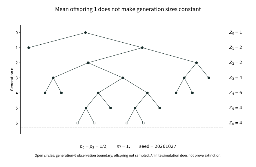
A finite record of a critical Galton–Watson family. Every individual whose reproduction is observed has either 0 or 2 children with equal probability, so mean offspring is 1. The MT19937 seed is 20261027; reproduction is sampled generation by generation, left to right. Populations in generations 0 through 6 are 1, 2, 2, 4, 6, 4 and 4. Generation 6 shows births only; its offspring are not sampled. The finite figure neither proves critical extinction nor determines this family’s infinite future.
[Static SVG](../assets/visuals/batch16-20/finite-gw-family.en.svg) · [Vector PDF](../assets/visuals/batch16-20/finite-gw-family.en.pdf)
Generation 6 is an observation boundary, not a completed infinite tree. A record that remains nonempty at that boundary does not refute critical extinction. Shapes conditional on large size, encodings and geometric limits require later random-tree tools. Here we have established the relationship between discrete single-type families and descendant weighting, not promoted a finite picture into a CRT construction.
## Chapter 20 Epilogue: Survival need not follow the mean curve
A family's future involves two different scales. The generating function asks whether anyone will remain to reproduce; normalized population asks whether a surviving tree retains the proportion predicted by mean growth. The same fixed-point equation eventually connects them, but only after verifying preservation of expectation can their answers be identified.
Size bias did not change the reproduction experienced by an original family. It changed which trees we observe, exposing rare large families in proportion to their contributions to mean population. The spine realizes that weighting as an actual genealogical line. The logarithmic condition determines whether enormous reproduction along it repeatedly overwhelms the exponential scale.
Survival, population tending to infinity, and a positive limit on the mean scale are therefore separate assertions requiring separate proofs. Some families keep growing while remaining much smaller than the mean curve; others retain a stable positive random proportion even without a second moment. The power and limitations of expectation appear within the same genealogical structure.
Making all individuals in a generation reproduce together supplied a tidy generational clock. If births and waiting occur separately in real time, genealogy remains but its clock must change. How branching connects with random time is another part of the picture this model naturally leaves open.
## Sources, modern reconstruction and proof scope
Watson and Galton's [1875 original paper](https://math.uchicago.edu/~shmuel/Modeling/Galton%20Watson.pdf), Journal of the Anthropological Institute 4, 138–144, documents the surname problem, generational generating-function calculations and nonoverlapping-generation assumption. The independent construction, probability-space formulation and martingale arguments here are modern reconstructions; the original population discussion is not treated as a modern theorem.
Kesten and Stigum's [1966 paper](https://doi.org/10.1214/aoms/1177699266) treats multidimensional Galton–Watson limit theory. Lyons, Pemantle and Peres's [1995 paper and public author version](https://arxiv.org/html/math/0404083v1) illuminate logarithmic criteria through size-biased trees. We checked our single-type supercritical route against its population weighting, infinite-level mass decomposition, spine immigration and Borel–Cantelli structure. Our decomposition is proved through a common dominating measure, and finite-logarithmic-moment immigration through submartingale convergence after fixing the sequence; exposition and organization are independently written.
The proved scope is strictly the single-type \(1
Divide an interval of length t into n cells, independently allowing an arrival in each with probability λt/n. Here λ>0 and n is sufficiently large. Chapter 13 gives a Poisson approximation for the total number. To study the first and second half-hours together, however, we must retain the locations of the cells, not merely the sum of all the Bernoulli variables.
\[
P\{N(t)=k\}=e^{-\lambda t}\frac{(\lambda t)^k}{k!},\qquad k=0,1,\ldots .
\]
This formula specifies only a one-time distribution. Writing it for every t does not specify how two times occur jointly. The consistency problem from Chapter 8 now has a concrete temporal form. We could start with shrinking cells, but would still have to construct limiting paths and rule out infinitely many arrivals accumulating in finite time. A more direct route starts with the waits between successive arrivals.
Chapter 19 has already constructed a general renewal process: when one wait ends, draw the next independently. But a new cycle is not the same thing as a new time. If every wait lasts exactly one hour, having already waited fifty minutes is crucial information. Independence between renewal cycles does not make counts in arbitrary time windows independent.
For independence alone, use a nondegenerate renewal counterexample. Let iid waits be uniform on (1,2). Almost surely there is exactly one arrival by time2, falling in (0,3/2] or (3/2,2] with probability1/2 each. The two events of one arrival are mutually exclusive, with joint probability0 rather than1/4. Independence of renewal cycles truly does not imply independence of time windows.
## 21.2 Can elapsed time cease to matter?
Let W be a strictly positive, almost surely finite wait, and write B(t)=P(W>t). Given that s units have elapsed without an arrival, the probability of waiting another t is B(s+t)/B(s). To reuse the original waiting rule whenever the clock is inspected, this ratio must equal B(t). Memorylessness means precisely this requirement, not a philosophical claim that the future has no causes.
\[
P(W>s+t\mid W>s)=P(W>t),\qquad s,t\ge0,\quad P(W>s)>0.
\]
First consider what it excludes. If W is uniform on (0,1), then for 0≤s<1 and 0≤t<1−s the conditional probability above is (1−s−t)/(1−s). It depends on s. The maximum possible duration restricts the future: an older cycle cannot continue waiting in the same way as a new cycle.
The requirement determines the distribution uniquely. Since W>0, B(h) tends to1 as h decreases to0 and is positive near0. Subdivide any t into sufficiently small pieces and apply memorylessness repeatedly to obtain B(t)=B(t/n)ⁿ>0. Thus the conditional probability is defined for every finite s, and B(s+t)=B(s)B(t).
\[
g(t)=-\log B(t),\qquad g(s+t)=g(s)+g(t),\qquad g(t)\ge0.
\]
The function g is nondecreasing. Set λ=g(1). Additivity first gives g(q)=λq for nonnegative rational q. Rational approximation from both sides and monotonicity give g(t)=λt for every real t≥0. Almost sure finiteness of W forces B(t)→0 and excludes λ=0. Thus strictly positive, almost surely finite memoryless waits are exactly exponential waits of rate λ>0. Substitution proves the converse. A density was not assumed; it is a conclusion.
\[
B(t)=e^{-\lambda t},\qquad f_W(t)=\lambda e^{-\lambda t}\mathbf1_{(0,\infty)}(t),\qquad EW=\frac1\lambda.
\]
The mean follows from Chapter 6’s tail-integral formula. If W=∞ is allowed, λ=0 can describe an arrival that never occurs; it is not a finite waiting distribution. The geometric distribution is memoryless on an integer clock, but embedding it in real time does not make the identity hold for all real s and t. The clock itself participates in selecting the law.
## 21.3 Constructing the entire arrival record
On the countable product probability space established in Chapter 8, take independent identically distributed exponential waits W₁,W₂,…. Join them end to end. Set S₀=0 and Sₙ=W₁+⋯+Wₙ, and let N(t) count the completed waits by t. The endpoint convention matters: an arrival occurring exactly at t has already been counted.
\[
N(t)=\sum_{n\ge1}\mathbf1_{\{S_n\le t\}},\qquad \{S_n\le t\}=\{N(t)\ge n\}.
\]
We must first prove that the sum is finite at finite t. Fix δ>0. The independent events {Wₙ≥δ} all have probability e^(−λδ)>0. The independent direction of Borel–Cantelli from Chapter 7 ensures infinitely many such events almost surely. Each contributes at least δ to the sums, so Sₙ→∞. Strict positivity of all waits holds on one common event of probability1, since only countably many null events must be excluded.
From now on restrict the probability space to this measurable full-probability subspace, with its trace σ-algebra and restricted probability. All finite-dimensional independent laws are unchanged, while every bounded interval now has finitely many arrivals for every sample. Paths of N are nondecreasing and right-continuous, have left limits, jump only by1, and start at0. These are simple, locally finite counting paths. Each N(t) is a measurable countable sum, and the event identities relating partial sums Sₙ to counts hold everywhere. This treatment makes later stopping-time arguments in the raw natural filtration independent of an unstated completion. Nonexplosion has been proved, not hidden inside max.
The waits are the construction material, arrival times their cumulative sums, and the step count another reading of the same record. They are not three unrelated models. We must now prove that this record produces the window laws we sought.
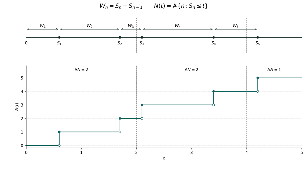
**Three expressions of one record.** Waits are0.6,1.1,0.4,1.3,0.8, giving arrival times0.6,1.7,2.1,3.4,4.2. Counts in (0,2], (2,4], (4,5] are2,2,1. Filled dots select the post-jump value; open dots mark the excluded pre-jump value. These are deterministic illustrative data, not a sampled Poisson record or a proof of independent increments. The unshown next wait is unfinished. The [vector publication PDF](../assets/visuals/poisson-time/arrival-record.pdf) and SVG share the same exact parameters.
## 21.4 A cancellation on the ordered-time region
Fix t>0 and require exactly n arrivals. If their locations are 0t)=e^(−λt) directly.
The ordered region has volume tⁿ/n!. Partition the cube (0,t)ⁿ into n! strict coordinate orders; diagonals have volume0. Alternatively, integrate Vₙ(t)=∫₀ᵗVₙ₋₁(s)ds inductively from V₀=1. Integrating the constant density gives the Poisson mass function. No process limit has been assumed.
\[
P(N(t)=n)=e^{-\lambda t}\frac{(\lambda t)^n}{n!},\qquad EN(t)=\lambda t,\quad \operatorname{Var}N(t)=\lambda t.
\]
The mean and variance follow by differentiating the exponential series or using Chapter 13’s generating function. The mean λt is a consequence of construction, and λ acquires its meaning as an arrival rate per unit time. It does not say that every path grows at constant speed on every small interval.
## 21.5 Why separate windows really are independent
Calculating N(t) is not enough. Take 0=t₀0 can therefore be constructed from exponential waits, or described as a count starting at0 with independent stationary Poisson increments. For λ=0, take the identically zero process. Homogeneity means that time translation does not change increment laws. Independent arrivals whose rate changes with time are not this homogeneous model.
The shrinking Bernoulli-cell idea now has a precise role. For finitely many fixed windows, subdivide each into finer cells and independently assign success probability λΔ to a cell of length Δ. Chapter 13 gives the appropriate Poisson limit for each binomial count. Joint masses across windows are products and converge to the displayed formula. This explains a finite-dimensional rare-event approximation, not path-space convergence. Paths were established separately by the waiting construction.
Except where the zero-rate case is discussed explicitly, take λ>0 below and retain the simple right-continuous path convention. The object is the joint law of a whole process, not a separately chosen Poisson random variable for each time.
## 21.6 The past contains more than the last count
At time s we may have observed every earlier arrival location, not just N(s). Let Fₛ⁰=σ(N(u):0≤u≤s), the raw natural filtration. Independence of the future from the past requires independence of future increment vectors from the whole of Fₛ⁰. Independence from N(s) alone is insufficient.
Fix future times 0≤v₁<⋯
Forget exponential waits. Assume only that N starts at0, has simple, locally finite, right-continuous nondecreasing integer paths on a common event of probability1, and has independent stationary increments. Must we additionally specify a Poisson law? The passage from single arrivals to a short-time probability law contains a step that needs proof.
Set q(t)=P(N(t)=0). Monotonicity and independent stationary increments give q(s+t)=q(s)q(t). Right-continuity and N(0)=0 imply N(h)→0 almost surely, hence q(h)→1. As in the waiting proof, q is positive at finite t, and monotone multiplicativity gives q(t)=e^(−λt) for a finite λ≥0. Only empty-window probabilities have been identified; clusters have not yet been ruled out.
Write p₂(h)=P(N(h)≥2) and n=⌊1/h⌋. A locally finite simple path has finitely many distinct arrivals in [0,1]. Their minimum separation is positive, with no minimum needed for fewer than two arrivals. For small enough h, no cell of length h contains two. Let Bₕ mean that one of the first n cells contains at least two. Its indicator tends to0 pathwise. Dominated convergence gives P(Bₕ)→0, while window independence gives an exact identity.
\[
P(B_h)=1-[1-p_2(h)]^{\lfloor1/h\rfloor}\longrightarrow0,\qquad p_2(h)=o(h).
\]
To check the last conclusion, if n p₂(h)≥ε>0 along a subsequence, then (1−p₂(h))ⁿ≤e^(−ε), a contradiction; now use nh→1. Thus one arrival has probability λh+o(h), while two or more have probability o(h). Simple paths have genuinely excluded batch jumps rather than merely supplied an attractive step diagram.
\[
P(N(h)=0)=1-\lambda h+o(h),\qquad P(N(h)=1)=\lambda h+o(h).
\]
For 0≤z≤1, put Gₕ(z)=E zᴺ⁽ʰ⁾, with 0⁰=1. The contribution from at least two arrivals is at most p₂(h), so Gₕ(z)=1−λh(1−z)+o(h). Divide fixed t into m equal windows. Independent stationary increments give Gₜ(z)=Gₜ/ₘ(z)ᵐ. Consequently:
\[
G_t(z)=\lim_{m\to\infty}\left[1-\frac{\lambda t(1-z)}m+o(m^{-1})\right]^m=e^{-\lambda t(1-z)}.
\]
Generating-function uniqueness from Chapter 13 identifies Poisson(λt), and independent increments determine all finite-dimensional laws. This proves the converse. For λ=0, counts at rational times are almost surely0; a countable intersection and right-continuity make the whole path zero. Allow jumps of size2 and N=2Q for a Poisson process Q retains independent stationary increments but loses Poisson counts. Simplicity cannot be discarded.
## 21.8 Identical Poisson marginals can hide different temporal relations
Even simple right-continuous paths do not let one-time laws imply independent increments. Couple all times through a single random number. Take U uniform on (0,1), let Fₖ(t) be the Poisson(t) cumulative distribution, and define a common-quantile process. The strict inequality chooses the right-continuous value at jumps.
\[
F_k(t)=e^{-t}\sum_{j=0}^k\frac{t^j}{j!},\qquad \widetilde N(t)=\min\{k\ge0:F_k(t)>U\}.
\]
For fixed t, P(Ñ(t)≤k)=Fₖ(t), so the marginal is Poisson(t). For fixed 0Fₖ(t) for t>0. The roots of Fₖ(t)=U increase strictly. They cannot accumulate at finite T because Fₖ(T)→1>U. These too are simple, locally finite, right-continuous counting paths.
\[
P\{\widetilde N(1)=0,\widetilde N(2)=1\}=e^{-1}-e^{-2}\ne e^{-2}=P\{N(1)=0,N(2)=1\}.
\]
The left side intersects (0,e⁻¹) with [e⁻²,3e⁻²) for U, since 3e⁻²>e⁻¹. The right side is the product for independent unit windows containing0 and1 arrival. The issue is neither whether a path can be drawn nor whether each marginal is correct, but how randomness at distinct times is jointly arranged.
## 21.9 Recovering independent waits from the count record
The converse gives all finite-dimensional count laws, but independence of the waits must still be recovered. An exponential empty-window probability determines only the first wait. To avoid borrowing a general continuous-time strong Markov theorem, use the countable-coordinate uniqueness from Chapter 8.
Restrict the given process and the process constructed in Section3 to nonnegative rational times. Equal finite-dimensional laws give equal laws on the countable product space: cylinders form a π-system, and measure uniqueness extends equality to the product σ-algebra. Each arrival time is a measurable function of these rational coordinates.
\[
S_n=\inf\{q\in\mathbb Q_{\ge0}:N(q)\ge n\},\qquad \inf\varnothing=\infty.
\]
Measurability follows from {Sₙ0, P(N(t)
The cancellation in Section4 leaves another piece of information. Given N(t)=n≥1, divide the arrival density by the event probability. The rate λ disappears. The conditional joint density is the constant n!/tⁿ on the ordered simplex.
\[
f_{S_1,\ldots,S_n\mid N(t)=n}(\mathbf s)=\frac{n!}{t^n}\mathbf1_{\{0
At deterministic s, the residual wait is Rₛ=S_{N(s)+1}−s. For r≥0, {Rₛ>r} is the event that (s,s+r] is empty. Section6 proves independence from Fₛ⁰, so the conditional tail is e^(−λr). This is stronger than the algebraic identity for one exponential wait: the entire observed record does not improve this prediction.
\[
P(R_s>r\mid\mathcal F_s^0)=e^{-\lambda r},\qquad E(R_s\mid\mathcal F_s^0)=\frac1\lambda.
\]
The renewal viewpoint also explains why the exponential law is special. Suppose an ordinary renewal process with strictly positive finite iid cycles and Sₙ→∞ starts at0 and has independent stationary increments. Its empty-window probability P(N(t)=0)=P(W₁>t) is multiplicative. Section2 forces the exponential waiting law. The converse is already proved. In this precise setting exponential renewal and independent stationary increments are equivalent; the word restart does not establish it.
Memorylessness does not eliminate Chapter 19’s length bias. A stationary exponential renewal interval seen from a typical time still has length-biased density λ²ℓe^(−λℓ) and mean2/λ, whereas an arrival-sampled cycle has mean1/λ. At a typical time, age and residual life are independent Exp(λ): Chapter 19’s joint density f(a+r)/μ becomes λ²e^(−λ(a+r)), which factors on a,r>0. A fresh-looking residual does not make the whole interval containing the observer a fresh cycle.
That paragraph concerns Chapter 19’s stationary construction, not the full age law at finite s for a process started at0; the latter may still be in its first wait. Initial conditions differ. The future may forget age while the entire observed cycle remains biased toward longer lengths.
## 21.12 What fairness remains after subtracting the mean count?
The count only increases and cannot itself be a fair game. But expected arrivals in a fixed-length future window equal λ times its length, unaffected by observed history. Subtracting that deterministic growth gives a continuous-clock instance of Chapter 15’s conditional fairness.
\[
M_t=N(t)-\lambda t,\qquad E(M_t\mid\mathcal F_s^0)=M_s,\quad 0\le s\le t.
\]
M is adapted, integrable at each time and right-continuous. Write Mₜ as Mₛ plus N(t)−N(s)−λ(t−s), then use Section6’s independence and mean; no Doob–Meyer decomposition is used. With Δ=N(t)−N(s), independence and VarΔ=λ(t−s) give E[(Δ−λ(t−s))²|Fₛ⁰]=λ(t−s), while the cross term has conditional mean0.
Here the martingale definition from Chapter 15 is used for all real 0≤s≤t: integrability at each time, adaptation and the conditional-mean identity. Replacing integer parameters by real ones does not automatically transfer every discrete-time theorem. We only prove directly that these two particular processes satisfy the definition.
\[
E\bigl(M_t^2-\lambda t\mid\mathcal F_s^0\bigr)=M_s^2-\lambda s,\qquad EM_t^2=\lambda t.
\]
Thus Mₜ²−λt is also a martingale. Centering leaves fluctuations whose second moments accumulate linearly in time. We establish this particular compensated counting martingale, not general stochastic integration or general compensation theory.
Fairness still depends on information. If the observer learns at time0 that no arrival will occur by t₀ and this future event enters the initial σ-algebra, then on that event Mₜ₀=−λt₀. Its conditional expectation cannot remain M₀=0. The process law has not changed, but the martingale property has because of advance information. Compensated fairness is not detached from a filtration.
## 21.13 Restarting at a time chosen by observation
Deterministic-time restart does not explain observing again after the third arrival. The record chooses this time. We prove the stopping property for the constructed Poisson process without invoking the next chapter’s general continuous-time Markov theory. Let τ be an almost surely finite stopping time for Fₜ⁰ and define Fτ by Chapter 16’s event condition.
On the possible null event {τ=∞}, define post-stopping increments and N(τ) to be0. Future identities are almost sure identities, with no subtraction ∞−∞. The grid sums below cover {τ<∞}, an event of probability1.
\[
\mathcal F_\tau^0=\{A\in\mathcal F_\infty^0:A\cap\{\tau\le t\}\in\mathcal F_t^0\text{ for every }t\ge0\},\qquad \mathcal F_\infty^0=\sigma\!\left(\bigcup_{t\ge0}\mathcal F_t^0\right).
\]
Approximate τ from above by dyadic times τₘ=2⁻ᵐ⌈2ᵐτ⌉. Each is a stopping time and τₘ↓τ. For A∈Fτ, A∩{τₘ=jh} belongs to Fjh, with h=2⁻ᵐ: for j≥1 it is the difference between A∩{τ≤jh} and A∩{τ≤(j−1)h}; for j=0 use {τ=0}. Apply deterministic-time independence on each grid event and sum over j.
\[
E\!\left[\mathbf1_A f\bigl(N(\tau_m+v_i)-N(\tau_m):1\le i\le k\bigr)\right]=P(A)\,E f\bigl(N(v_i):1\le i\le k\bigr).
\]
The grid sum is absolutely bounded by ‖f‖∞ΣP(A∩{τₘ=jh}), so an unbounded finite τ is harmless. Right-continuity on one common path event gives N(τₘ+vᵢ)→N(τ+vᵢ) and N(τₘ)→N(τ). A convergent finite integer-valued vector is eventually equal to its limit. Every bounded Borel f therefore converges pathwise, without needing continuity. Dominated convergence gives the identity with τ in place of τₘ.
Thus post-τ increments are independent of Fτ and have the original process law; π–λ extends finite future cylinders to all future coordinates. Measurability of N(τ) can be checked: {N(τ)≥j}={τ<∞,Sⱼ≤τ}. Intersecting with {τ≤t} gives {Sⱼ≤t}∩{τ≤t}∩{Sⱼ∧t≤τ∧t}, all in Fₜ⁰. The current count at stopping really belongs to the stopping information.
Every Sⱼ is a stopping time since {Sⱼ≤t}={N(t)≥j}. Independent restart holds not only at arrivals but at every finite stopping time in the stated class. This includes neither restarting after infinity nor treating times selected retrospectively using the future as stopping times. The information direction agrees with Chapter 16.
## 21.14 Why independent coloring separates independent streams
An arrival may also carry a type. Let the types be independent of the arrival process and drawn independently with probabilities p₁,…,pᵣ, where Σpᵢ=1. Multiply the original space by a countable iid mark space. Let Nᵢ(t) count type-i arrivals. Independent marking concerns the whole type sequence, not just marginal proportions.
In a window of length h, type counts conditional on the original total n are multinomial. For k₁+⋯+kᵣ=n, multiply the Poisson and multinomial masses; the n! factors cancel. A type of probability0 has no arrivals, with 0⁰=1 in the formula.
\[
P\{N_i(s+h)-N_i(s)=k_i,\ 1\le i\le r\}=\prod_{i=1}^r e^{-\lambda p_i h}\frac{(\lambda p_i h)^{k_i}}{k_i!}.
\]
Different windows must also be checked. Conditional on all original arrival locations, disjoint windows select disjoint sets of mark indices, determined only by the arrival record and independently of the marks. Conditional allocations across windows are independent and depend only on their respective totals. Integrating against the independent Poisson window totals factors the joint mass across every window and color. Cylinder uniqueness gives r independent processes with rates λpᵢ.
This is independent thinning. Retaining one color with probability p leaves rate λp. Coloring odd arrivals red and even arrivals blue violates the assumptions: same-color successive gaps sum two exponential waits, and colors must alternate. Apparent half-and-half proportions cannot replace independent marking.
## 21.15 Why merging preserves the process
Take finitely many independent Poisson processes with rates λ₁,…,λᵣ and put N=ΣNᵢ. A bounded interval has finitely many arrivals in total. Disjoint-window increments are independent, being built from independent window variables within independent processes. Chapter 13’s generating-function calculation makes each window total Poisson with the sum of the rates.
\[
\Lambda=\sum_{i=1}^r\lambda_i,\qquad E z^{N(t)}=\prod_{i=1}^r e^{-\lambda_i t(1-z)}=e^{-\Lambda t(1-z)}.
\]
Simplicity also requires excluding simultaneous arrivals. The nth and mth arrival times of two positive-rate processes are independent with continuous densities, so their equality has probability0; Fubini verifies this by conditioning on one time. The union over finitely many process pairs and countably many n,m is still null. Zero-rate processes have no arrivals. The merged process is a simple Poisson process.
Independence cannot be omitted from merging. Adding the same Q twice gives N=2Q, with jumps of size2 and only even values, although EN(t)=2λt. Rates may add at the mean level without producing a Poisson model. This is the same structural distinction as Chapter 13’s clustered-event counterexample to independent rare-event approximation.
## 21.16 A linear long-run rate does not mean evenly spaced arrivals
Exponential waits have finite mean1/λ. Chapter 12’s integrable iid strong law gives Sₙ/n→1/λ. Since S_{N(t)}≤t0, P(Wₙ>ε)=e^(−λε) does not shrink with n; independence makes waits exceeding any fixed length occur infinitely often. A long-run average allows irregular local spacing. The compensated martingale variance λt identifies a √t second-moment fluctuation scale. A path limit still requires the later function-space theory.
Another boundary is a nonhomogeneous clock. The deterministic time change N(t)=Q(t²) of a rate1 process Q retains independent increments, but the expected count in (s,s+h] is2sh+h², not a function of h alone. It is not a homogeneous Poisson process and lacks exponential waits of one constant rate. Independence and stationarity of increments are distinct assumptions.
## 21.17 When clocks compete, which one changes the state?
Streams can merge, and waiting clocks can compete directly. Take independent Eᵢ∼Exp(λᵢ), initially all λᵢ>0. Let H=minEᵢ and J identify the first clock to ring. Continuity excludes ties. Multiplying survival probabilities gives P(H>t)=exp(−Λt), but the first type needs a joint calculation.
\[
P\{H\in dt,J=i\}=\lambda_i e^{-\lambda_i t}\prod_{j\ne i}e^{-\lambda_jt}\,dt=\lambda_i e^{-\Lambda t}\,dt.
\]
Integration gives P(J=i)=λᵢ/Λ; the joint density factors into an Exp(Λ) density times this probability, so H and J are independent. For λᵢ=0, place that clock at∞; the conclusion remains valid when Λ>0. If all rates vanish there is no next ring, and λᵢ/Λ is not a probability.
This factorization changes the description of a system. While its state stays fixed, draw a total wait and then choose a change type according to relative rates. An arrival that changes state may change the next rates. Global counts need no longer have independent stationary increments, and finite-time accumulation must be reconsidered. Exponential competition gives a next-step rule without yet constructing a general continuous-time chain.
## 21.18 What a memoryless model does, and does not, explain
We began with a one-hour total. The same object can now be read as independent waits, ordered arrival times, or joint counts over all time windows. They are connected not by the name Poisson but by two compatible restarts we have proved: drawing a fresh wait after an arrival and continuing from an observed time. Exponential memorylessness makes these agree; independent stationary increments express that agreement in the law of an entire record.
The structure is strong, and its boundaries are clear. Independent cycles, correct marginals, a constant mean rate or suitable color proportions are not enough. Age, a shared environment, batch arrivals and advance information can each change one of the relations. Memorylessness is a precise, testable model property, not a declaration about every real-world wait.
When a ring merely increases a count by1, the rate stays unchanged. If it breaks a machine, brings a birth or changes the system’s state, the next wait is determined by the new state. We know how to wait within a state. The next task is to understand how states and clocks together form a random path that actually exists.
## Sources, proof provenance and scope
Robert Gallager’s original MIT course notes, [Poisson Processes](https://ocw.mit.edu/courses/6-262-discrete-stochastic-processes-spring-2011/resources/mit6_262s11_chap02/), provide a technical comparison for waits, counts, independent increments and splitting; the [chapter PDF hosted by the author’s institution](https://www.rle.mit.edu/rgallager/documents/Poisson.pdf) makes the discussion verifiable. We reorganize the mathematics around our preceding problems and develop proofs independently. We neither reproduce the notes nor attribute modern product spaces, filtrations and π–λ arguments to Poisson’s original discoveries. The process’s name does not establish a claim about its entire historical origin.
Established prerequisites are [infinite experiments in Chapter 8](08-infinite-experiments.md), [rare counts and generating functions in Chapter 13](13-rare-events.md), [stopping information in Chapter 16](16-stopping-times.md), and [renewal and typical times in Chapter 19](19-renewal.md). General state changes, spatial point processes, random intensities and stochastic integration do not follow automatically from these count calculations. A finite figure explains different expressions of one record, not an infinite-time conclusion.
---
# Chapter 22: How Can a Random Process Jump?—Continuous-Time Markov Chains
A machine fails and repair begins. There is no reason for the wait to failure and the wait to repair to have the same rate. After repair, the failure clock starts again. With several machines, one clock ringing may even change the operating conditions of the others. Each change is simple, but one fixed-rate counting process no longer describes the whole record.
Growth raises a more troubling possibility: more individuals mean a faster next birth. If a system accelerates indefinitely, can strictly positive waits all be exhausted in finite time? Before asking about a long-run distribution, we must determine how far the path specified by local rules actually exists.
## 22.1 Separating how long to wait from where to go
For a machine with working and repair states, wait an Exp(a) time while working and enter repair; wait Exp(b) during repair and return to work. With several possible changes from a state, the exponential race of Chapter 21 says to add their rates for the total wait, then choose the destination in proportion to the rates.
A local rule at state i therefore contains an exit rate qᵢ and destination probabilities rᵢⱼ. Combining them as qᵢⱼ=qᵢrᵢⱼ records both waiting and direction. A ring that leaves the state unchanged should not count as an actual jump. Otherwise arbitrary invisible rings would assign different exit rates to the same visible path.
\[
q_{ij}\ge0\ (j\ne i),\qquad q_i=\sum_{j\ne i}q_{ij}<\infty,\qquad q_{ii}=-q_i.
\]
We work on a finite or countable state space E with its discrete σ-algebra. The display defines a stable conservative rate matrix Q. Stable means each qᵢ is finite, not that all rates have a common bound. Conservative means row sums are zero, not that nonexplosion has already been proved. A state with qᵢ=0 is absorbing. Direct killing in a sub-conservative matrix can be represented by a cemetery extension; we do not conflate those assumptions here.
## 22.2 Joining local rules into a record
Enumerate E once and for all. For qᵢ>0 set rᵢⱼ=qᵢⱼ/qᵢ for j≠i and rᵢᵢ=0; for qᵢ=0 set rᵢᵢ=1. Independent uniforms successively select Y₀,Y₁,… from these rows. This embedded chain records destinations while suppressing the waits. Inverse cumulative allocation on a countable space is measurable. The construction uses the countable experiments of Chapters 8 and 10, without hiding the extra difficulties of arbitrary measurable state spaces.
Independently of the whole embedded chain, take iid Exp(1) variables E₀,E₁,…. Here Eₙ is a random variable and E is the state set. Rescale the unit clocks by the current rate: Hₙ=Eₙ/q_{Yₙ}, taking Hₙ=∞ at a zero rate. Set T₀=0 and Tₙ=Σₖ₌₀ⁿ⁻¹Hₖ. After an infinite wait, all subsequent T values are∞; no subtraction ∞−∞ is performed.
\[
\zeta=\lim_{n\to\infty}T_n,\qquad
X_t=\begin{cases}Y_n,&T_n\le t
Fix t before explosion and partition the history by the number n of completed jumps. If Yₙ=i, the history determines H₀,…,Hₙ₋₁ and reveals Hₙ>t−Tₙ. It has not seen the next uniform destination choice or later clocks. Conditional on the entry time and those past data, exponential memorylessness restores an Exp(qᵢ) residual wait, independent of the unused destination choice.
The argument also handles random age. First integrate simple functions of the entry time and finite historical coordinates against their independent product law, obtaining conditional tail e^(−qᵢs); extend by a monotone class. Sum over n. The conditional future law depends only on i; after explosion the future is constantly Δ. With Fₜ⁰=σ(Xᵤ:0≤u≤t), every bounded future cylinder function G satisfies:
\[
E_i[G(X_{t+s_1},\ldots,X_{t+s_k})\mid\mathcal F_t^0]
=E_{X_t}[G(X_{s_1},\ldots,X_{s_k})].
\]
This proves the Markov property from construction. Put pᵢⱼ(t)=Pᵢ(Xₜ=j) for i,j∈E. Its row sum is Pᵢ(ζ>t), possibly below1; on E∪{Δ} the transition law is a full probability. Conditional averaging and nonnegative summation give Chapman–Kolmogorov.
\[
p_{ij}(t+s)=\sum_{k\in E}p_{ik}(t)p_{kj}(s),\qquad P(0)=I.
\]
Short-time rates must also be checked from paths. Starting from fixed i, after a first jump to k the chance of another jump within h is at most1−e^(−qₖh). Thus two or more real jumps have probability at most hΣₖ≠ᵢqᵢₖ(1−e^(−qₖh))=o(h), by dominated convergence using Σqᵢₖ=qᵢ<∞. Exactly one jump to j followed by no further jump has probability ∫₀ʰe^(−qᵢs)qᵢⱼe^(−qⱼ(h−s))ds.
\[
p_{ij}(h)=q_{ij}h+o(h)\ (j\ne i),\qquad
p_{ii}(h)=1-q_i h+o(h).
\]
Each remainder concerns fixed i,j. It cannot be summed uniformly over an unbounded state set without proof. Correct derivatives for individual rows do not grant unrestricted differentiation and multiplication of infinite matrices.
## 22.4 Can the process restart at a time chosen by observation?
For this constructed jump chain, the method of Chapter 21 independently proves stopping restart. Let τ be an almost surely finite stopping time for the raw natural filtration, with Fτ defined by its event condition and fixed conventions on the null infinity slice. Set τₘ=2⁻ᵐ⌈2ᵐτ⌉. For A∈Fτ, its slice on {τₘ=j2⁻ᵐ} belongs to the information at that grid time.
\[
E_i[\mathbf1_A G(X_{\tau_m+s_1},\ldots,X_{\tau_m+s_k})]
=E_i[\mathbf1_A\,g(X_{\tau_m})],\qquad
g(x)=E_xG(X_{s_1},\ldots,X_{s_k}).
\]
Boundedness controls the countable grid sum. Right-continuity and discrete states make each finite collection X_{τₘ+s},X_{τₘ} eventually equal its limit, including Δ when τ=ζ. Dominated convergence applies on both sides, proving the specialized strong Markov property. Measurability of the stopped value follows by approximating X_{τ∧t} from above using τₘ∧t and its finite grid partition. Hence {τ≤t,Xτ=j} belongs to Fₜ⁰.
This was not borrowed from a general continuous-time regularization theorem. It uses right-continuity, discrete states and the explicit cemetery rule. In general state spaces, nearby times need not give eventually identical states; the additional tools belong to later path and semigroup theory.
## 22.5 Why expand according to the number of jumps?
For unbounded rates, writing an exponential series in Q may not even produce meaningful terms. Paths offer a safer expansion: first no jump, then exactly one, and so on. Let p⁽ⁿ⁾ᵢⱼ(t) be the probability of exactly n real jumps by t, no explosion and current state j.
\[
p^{(0)}_{ij}(t)=\delta_{ij}e^{-q_i t},\qquad
p^{(n+1)}_{ij}(t)=\int_0^t e^{-q_i s}\sum_{k\ne i}q_{ik}\,p^{(n)}_{kj}(t-s)\,ds,\qquad
p_{ij}(t)=\sum_{n=0}^\infty p^{(n)}_{ij}(t).
\]
The density of a first jump at s to k is e^(−qᵢs)qᵢₖ; the remaining interval has n further jumps. All terms are nonnegative, so Tonelli permits exchanging integrals and the sums over states and jump counts. Every path before ζ has finitely many jumps, so the final sum misses nothing and includes no mass reappearing after explosion.
Minimality has a precise equation meaning. If a nonnegative matrix function R satisfies the same first-jump integral equation, then R≥p⁽⁰⁾. Substitute again to get R≥p⁽⁰⁾+p⁽¹⁾, and inductively R≥Σₙ≤ₘp⁽ⁿ⁾. Monotone passage gives R≥P. If P has row sums1, any such R with row sums at most1 must equal P. Nonexplosion therefore also establishes uniqueness in this solution class.
## 22.6 Reading the backward equation from the first jump
Group the expansion by its first jump to obtain a backward integral equation without formal differentiation. Changing to the remaining-time variable u exposes the exponential convolution kernel.
\[
p_{ij}(t)=\delta_{ij}e^{-q_i t}
+\int_0^t e^{-q_i(t-u)}\sum_{k\ne i}q_{ik}p_{kj}(u)\,du.
\]
The inner sum is bounded by qᵢ. Even if initially only measurability is known, convolution with this exponential kernel is continuous: translated kernels converge in L¹ on bounded intervals, and short endpoint intervals contribute vanishing amounts. Thus all pₖⱼ are continuous. Domination by the summable fixed row qᵢₖ makes Σqᵢₖpₖⱼ continuous as well. Differentiation by the integrating factor is now justified.
\[
\frac{d}{dt}p_{ij}(t)=\sum_{k\in E}q_{ik}p_{kj}(t)
=-q_i p_{ij}(t)+\sum_{k\ne i}q_{ik}p_{kj}(t),\qquad P'(t)=QP(t).
\]
For each fixed i,j, the derivative is continuous for t>0, with a right derivative at0. The matrix shorthand P′(t)=QP(t) denotes precisely these entrywise identities; it makes no claim of differentiability in an operator norm for infinite matrices. The absolute row sum is at most2qᵢ. The equation is called backward because the decomposition begins at the initial state and its first jump, not because physical time runs backward.
## 22.7 Reading the forward equation from the last jump
Alternatively decompose at the final jump into j. A path with n+1 jumps first makes n jumps and is at k just before s, jumps to j at rate qₖⱼ, then remains there until t. Integrate the ordered path density over the last jump time and use Tonelli to sum, obtaining another rigorous integral equation.
\[
p_{ij}(t)=\delta_{ij}e^{-q_jt}
+\int_0^t e^{-q_j(t-s)}a_{ij}(s)\,ds,\qquad
a_{ij}(s)=\sum_{k\ne j}p_{ik}(s)q_{kj}.
\]
Now a column qₖⱼ is fixed and its sum may be infinite. The equation itself supplies integral control: on [0,T], the exponential factor is at least e^(−qⱼT), so ∫₀ᵀaᵢⱼ(s)ds≤e^(qⱼT). Thus, for each fixed i,j, pᵢⱼ is locally absolutely continuous and satisfies the following entrywise forward equation for Lebesgue almost every t; the matrix shorthand in the display has only this meaning.
\[
\frac{d}{dt}p_{ij}(t)=\sum_{k\in E}p_{ik}(t)q_{kj}
=a_{ij}(t)-q_jp_{ij}(t),\qquad P'(t)=P(t)Q\quad\text{a.e.}
\]
For general unbounded rates, the result here is the integral equation and the almost-everywhere differential equation; we do not enlarge the scope by saying standard differentiation. If supₖ≠ⱼqₖⱼ is finite for a fixed j, then aᵢⱼ is continuous and the equation holds for every t>0. Indeed a deterministic time is almost surely neither a jump nor an explosion: the first wait has a continuous density, and conditioning on the first destination convolves it with each later jump time or lifetime, leaving no finite atoms. Paths are then locally constant on both sides of deterministic t almost surely, giving total-variation continuity of transition rows. A bounded column can be passed through that limit.
In particular, a common bound on all exit rates bounds every column. The forward equation describes inflow and outflow; the backward equation unfolds the initial state. For finite matrices both are familiar ODEs. In infinite state spaces the summability justifications differ.
## 22.8 One fast clock can contain many slower clocks
If supᵢqᵢ≤c<∞, use a rate-c Poisson clock. At each ring choose a state using R=I+Q/c, allowing a self-step. These virtual jumps deliberately unify the clock and must not be confused with real jumps of the embedded chain. If c=0 every state is absorbing; take c>0 below.
\[
P(t)=e^{-ct}\sum_{n=0}^{\infty}\frac{(ct)^n}{n!}R^n,\qquad R=I+\frac Qc.
\]
At state i, each independent virtual choice accepts a real exit with probability qᵢ/c. Chapter 21’s thinning proof makes the first real wait Exp(qᵢ), with accepted destination j of probability qᵢⱼ/qᵢ. After geometrically many failures, unused choices and the future clock remain independent, successively reproducing Section2’s construction. Finitely many rings in bounded time imply nonexplosion.
The matrix series converges in operator norm on bounded functions because R has sup-norm operator norm1. Its derivative series converges uniformly on compact time intervals by exponential-series bounds. Both differential equations therefore hold pointwise, with a unique solution equal to the bounded-operator exponential e^(tQ). This provides a practical finite-chain calculation and identifies what unbounded rates lack: a common clock of finite speed.
## 22.9 How infinitely many positive waits fit into finite time
For0<λₙ<∞, a pure-birth chain moves through i,i+1,i+2,…, waiting an independent Exp(λₙ) time at n. Its embedded chain is deterministic, so the entire difficulty lies in the clock. With independent Exp(1) variables Eₙ, its lifetime is Σₙ≥ᵢEₙ/λₙ.
\[
\sum_{n\ge i}\lambda_n^{-1}<\infty\quad\Longrightarrow\quad
E_i\zeta=\sum_{n\ge i}\lambda_n^{-1}<\infty\quad\Longrightarrow\quad
P_i(\zeta<\infty)=1.
\]
The converse cannot say that infinite mean forces an infinite random variable; Chapters 7 and 12 have already shown why that fails. Use independence through the Laplace reading of the whole sum. Multiply over finite partial sums and then apply bounded convergence to their exponentials:
\[
E_i e^{-\zeta}=\prod_{n\ge i}\frac{\lambda_n}{1+\lambda_n}
=\exp\!\left[-\sum_{n\ge i}\log(1+\lambda_n^{-1})\right],\qquad e^{-\infty}=0.
\]
If Σ1/λₙ=∞, either infinitely many reciprocals are at least1, repeatedly adding at least log2, or eventually they are below1 and log(1+x)≥x/2 makes the logarithmic sum diverge. Thus E e^(−ζ)=0, forcing ζ=∞ almost surely. Divergence of Σ1/λₙ is exactly nonexplosion for a pure-birth chain; convergence is almost sure explosion.
Rates λₙ=λn accelerate only at the harmonic threshold and do not explode, whereas λₙ=2ⁿ give finite mean lifetime. Every individual wait is positive, every qₙ finite and every row conservative, yet accumulation still occurs in the latter case. This simplest path already separates local validity from global lifetime.
## 22.10 After explosion: a rule absent from the matrix
Take E={0,1,2,…} with qₙ,ₙ₊₁=2ⁿ. The minimal process enters the cemetery after its finite lifetime, losing row mass within E. Alternatively, restart independently from0 after each explosion. Complete cycle lifetimes are iid and strictly positive, so Borel–Cantelli makes their sum diverge. Infinitely many complete cycles cannot accumulate in finite time.
A second version restarts at1 after every explosion. Both restarted records are Markov at deterministic times: inside a cycle, the past only censors the current exponential wait, whose residual and later cycles remain independent. Partition by cycle number and jump number within the cycle. Both paths are right-continuous but lack a left limit in discrete E at explosion.
They still have the same Q. From fixed i, explosion by h requires at least two independent waits, with probability at most (1−e^(−2ⁱh))(1−e^(−2ⁱ⁺¹h))=O(h²). Restart therefore does not alter any fixed-state short-time derivative. But from0, the restart-at1 version never returns to0 and has p₀₀(t)=e^(−t). Restart at0 adds the positive probability of an explosion followed by a restart with no further exit, making p₀₀(t) strictly larger for some t.
Positivity requires no guess about the lifetime density. Since ζ is finite almost surely, some finite t has P(ζ0. A first-cycle explosion before t is followed by a wait exceeding t−ζ with probability e^(−(t−ζ))>0. We do not claim these are nonexplosive E-valued càdlàg chains. The example shows that Q does not prescribe continuation across an explosion boundary. Minimal killing, or a prior proof of nonexplosion, restores the appropriate uniqueness.
## 22.11 Can explosion be ruled out without tracking every path?
Bounded rates are too restrictive: the nonexplosive pure-birth process with rates λn has unbounded rates. Seek a quantity limiting rapid escape to large states. Let V:E→[1,∞) have finite sublevel sets {Vmaxᵢ∈Fqᵢ with C_F>0, freeze all rows outside F at0, and apply Section8’s common clock. This local clock rate C_F differs from the growth constant c in QV≤cV. Each virtual jump has conditional mean V-increment QV/C_F, including the actual outside value at the exit. Finiteness of F and of each ΣqᵢⱼV(j) ensures absolute integrability over finite time: absolute change rates have a finite maximum on F.
Partition the clock into small cells, or sum over the ordered-time densities of its Poisson rings, to obtain expected increment as expected integrated rate. For the latter, Chapter 21’s density gives a ring at s with mean increment QV/C_F given the prior state and mean ring density C_F ds. First justify the exchanges for absolute increments by Tonelli, then subtract positive and negative parts. Thus:
\[
E_i V(X_{t\wedge\tau_F})
=V(i)+E_i\int_0^{t\wedge\tau_F} QV(X_s)\,ds.
\]
Expand that sum once more to remove any ambiguity about ring density. Let Jₙ be the nth ring of the rate-C_F clock, Cₙ the uniformized discrete state and K its first exit step from F. The density of Jₙ₊₁ is C_F e^(−C_Fs)(C_Fs)ⁿ/n!, independently of the whole C sequence; the conditional increment at step n+1 is QV(Cₙ)/C_F. The expected total increment is therefore ∫₀ᵗΣₙ≥₀e^(−C_Fs)(C_Fs)ⁿ/n! E[1_{nV(i).
\]
Finally, explosion must force exit from every finite F. During visits to F choose C≥max(1,maxᵢ∈Fqᵢ), so rates are bounded by C. Conditional on the whole embedded chain, infinitely many such indices carry independent unit clocks with a fixed positive probability of contributing at least1/C. Borel–Cantelli makes total waiting diverge. Take one common event for the countable sublevel sets. Thus {ζ≤t} is contained in every {τ_{V
For a birth-death chain with qₙ,ₙ₊₁=aₙ and qₙ,ₙ₋₁=bₙ, take V(n)=n+1. Then QV(n)=aₙ−bₙ≤aₙ. If aₙ≤c(n+1), the criterion gives nonexplosion regardless of the death rates, provided each bₙ is finite. Death pushes toward smaller states. Infinitely many downward jumps on nonnegative integers would require enough upward replenishment.
This upper bound on QV is not a classification of every explosion problem. Failure to find a suitable V means only that this criterion has not answered the question, not that explosion follows. The exact pure-birth criterion answers a necessary-and-sufficient question in a narrower model. A sufficient tool and a full characterization are different achievements.
## 22.13 Why balance equations require summability too
A probability π is invariant when πP(t)=π for every t. The forward equation suggests the algebraic flow balance πQ=0, but in infinite state spaces this should not replace the probability definition. Here is a precise equivalence: for a probability π with Σᵢπᵢqᵢ<∞, balance πQ=0 is equivalent to invariance of the minimal process.
\[
\sum_i\pi_iq_i<\infty,\quad \pi Q=0
\quad\Longleftrightarrow\quad \pi P(t)=\pi\quad(t\ge0).
\]
For sufficiency use the pointwise backward equation. For bounded f:E→R put Pₜf(i)=Eᵢ[f(Xₜ);t<ζ]. The same first-jump convolution gives dPₜf(i)/dt=Q(Pₜf)(i), bounded by2qᵢ‖f‖∞. The finite π-average exit rate permits differentiation through the π-sum. Fubini is then justified by Σᵢⱼπᵢ|qᵢⱼ|≤2Σπᵢqᵢ:
\[
\frac d{dt}\sum_i\pi_iP_tf(i)
=\sum_j\left(\sum_i\pi_iq_{ij}\right)P_tf(j)=0.
\]
The initial value gives invariance, and f=1 shows no cemetery loss under π. Conversely, if π is invariant, differentiate πPₜf at0 for coordinate indicators f=1ⱼ, using the same summable derivative bound, to obtain πQ=0. No signed infinite sum was treated as formal matrix algebra. For irreducible Q, a strictly positive invariant π also transfers nonexplosion from π to each initial state.
Finite mean rate is the condition supporting these exchanges, not a claim that every invariant probability must satisfy it. General invariance, boundary flux and infinite mean-rate cases belong to the broader process theory. The proved version here cannot be used after erasing its condition.
## 22.14 Jump-sampled and time-sampled states have different weights
The embedded chain records each visit once regardless of its duration. A clock observation gives longer waits more opportunity. This resembles Chapter 19’s length bias, but the weights now concern state holding times rather than entire renewal cycles. Suppose every qᵢ>0, R has invariant probability ν, and Z=Σᵢνᵢ/qᵢ is finite.
\[
\pi_i=\frac{\nu_i/q_i}{Z},\qquad
\sum_i\pi_iq_i=\frac1Z,\qquad
(\pi Q)_j=\frac1Z\left(\sum_{i\ne j}\nu_ir_{ij}-\nu_j\right)=0.
\]
Section13 proves that π really is invariant for the minimal process, rather than merely guessing a weight. Conversely, for invariant π with0<α=Σπᵢqᵢ<∞, setting νᵢ=πᵢqᵢ/α and using balance gives νR=ν. Absorbing states require separate treatment and cannot enter division by qᵢ.
The two-state machine alternates forever in its embedded chain, giving each state half the visits. Time weights are πworking=b/(a+b) and πrepair=a/(a+b). Slow repair still alternates one-for-one with working periods in the visit log, yet a random time is more likely to find repair. The probability laws do not conflict; the observation rule changed.
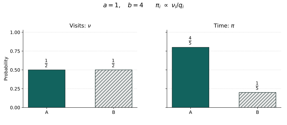
**Equal visits need not mean equal time.** Let A be working and B repair, with a=1,b=4. The left-hand halves come from alternating embedded visits; the right-hand four-fifths and one-fifth are proved stationary time weights from mean holds1 and1/4. They are not empirical frequencies of a finite simulation, and the figure does not prove convergence. Hatching and shading distinguish states in monochrome. The [vector PDF](../assets/visuals/jump-clocks/state-time-weight.pdf) shares exact parameters with the SVG.
## 22.15 Why continuous time removes a finite chain’s periodic obstruction
For finite irreducible Q, choose c>maxqᵢ so the uniformized matrix R=I+Q/c has positive diagonal entries. R is irreducible and aperiodic. Chapter 17 proved that Rⁿ converges to its unique invariant probability π. This π satisfies πQ=0 and is invariant for the continuous chain.
\[
\|P_i(t)-\pi\|_{\rm TV}
\le \sum_{n\ge0}e^{-ct}\frac{(ct)^n}{n!}\,\|R_i^n-\pi\|_{\rm TV}\longrightarrow0.
\]
Given ε>0, choose K so every discrete distance for n≥K is below ε. The remaining finite part is bounded by P(Poisson(ct)
Take λ>0 and let each individual independently give birth at rate λ, remaining alive afterward. With n individuals, exponential competition makes the next birth wait Exp(λn), with a uniformly chosen parent. The population Zₜ is a pure-birth chain with λₙ=λn. Section9’s harmonic criterion guarantees that infinitely many births cannot occur in finite time. Below Zₜ consistently denotes population.
Starting at1, the forward integral equation closes successively in n. We have p₁(t)=e^(−λt), and for n≥2, pₙ′=λ(n−1)pₙ₋₁−λnpₙ with pₙ(0)=0. Each state has only one incoming state, so no infinite-column exchange is needed. Induction by integrating factors, or substitution plus this successive uniqueness, gives:
\[
P_1(Z_t=n)=a(1-a)^{n-1},\quad n\ge1,\qquad
a=e^{-\lambda t},\qquad E_1Z_t=a^{-1},\quad E_1Z_t^2=\frac{2-a}{a^2}.
\]
The masses sum to1; moments follow by differentiating the geometric series. Construct descendants of z initial individuals independently and merge them. Exponential competition reproduces the same λn rule, so their total has the law of the pure-birth chain started at z. This establishes branching, rather than declaring family independence merely from linear population rates.
## 22.17 A population limit without borrowing future convergence theory
Branching and Markov properties give E(Zₜ|Fₛ)=Zₛe^(λ(t−s)), so Mₜ=e^(−λt)Zₜ is a martingale with EMₜ²=2−e^(−λt)≤2. Chapter 15’s discrete-time convergence theorem does not automatically cover every real time. This special model can instead be settled directly by Chapter 12’s random series.
\[
\lambda A_n=\sum_{k=1}^{n-1}\frac{E_k}{k},\qquad
\lambda A_n-\log n
=\sum_{k=1}^{n-1}\frac{E_k-1}{k}
+\left(\sum_{k=1}^{n-1}\frac1k-\log n\right)\longrightarrow L\in\mathbb R.
\]
Here Aₙ is the first time population reaches n, with A₁=0; the symbol Aₙ distinguishes it from the nth jump time Tₙ of Section2. The centered series has independent terms with summable variances Σ1/k², so Chapter 12’s proved series theorem gives almost sure convergence. The harmonic-logarithm difference converges by integral bounds and monotonicity. Therefore n e^(−λAₙ)→e^(−L)>0.
For Aₙ≤t0 along all real times on one event. The second-moment bound gives uniform integrability: E[Mₜ;Mₜ>K]≤EMₜ²/K≤2/K. Chapter 7’s Vitali criterion applied to every sequence tₘ→∞ gives L¹ convergence and EW=1.
\[
P(M_t>x)=(1-e^{-\lambda t})^{\lfloor xe^{\lambda t}\rfloor}
\longrightarrow e^{-x}\quad(x\ge0),\qquad W\sim{\rm Exp}(1).
\]
The exact geometric tail identifies the limit law. Survival here is certain, but the eventual random proportion is not. A mean growth curve does not specify what fraction one family will realize. This example’s second moments and explicit clock prevent mean loss, without erasing Chapter 20’s L log L obstruction for general families.
## 22.18 A reproduction may bring many children, or none
More generally, take β>0 and let each individual live an independent Exp(β) time and is replaced at death by K children, where P(K=k)=pₖ, K is a finite nonnegative integer and m=EK<∞. Children repeat the rule independently. With population z, reproduction completions have total rate βz and a uniform parent, changing population by K−1. When K=1 the population stays unchanged although a life replacement occurs; the population chain’s real exit rate is therefore not βz.
\[
q_{z,z-1+k}=\beta z p_k\quad(k\ne1),\qquad
q_z=\beta z(1-p_1),\qquad q_0=0.
\]
To construct the timed family itself, invisible one-child events cannot simply be discarded. Add J to count every reproduction completion. From (z,j), jump to (z−1+k,j+1) at rate βzpₖ, with z=0 absorbing. For V(z,j)=z+j+1, sublevel sets are finite and each increment is k, so QV=βzm≤βmV. Section11 proves nonexplosion of all reproduction events, not merely visible population changes.
At each event independently choose a uniform parent and attach finitely numbered children to the genealogy. Bounded time has finitely many events, each with finitely many children, giving a countable tree with defined birth and death times. Exponential competition and memorylessness identify this with assigning independent lifetimes and offspring numbers to individuals. Independent product constructions for distinct initial ancestors establish branching probabilistically.
The correspondence between independent lifetimes and uniform parent choice can be checked directly. For z independent Exp(β) clocks, specify clock i as first at s and require all other residual lifetimes to exceed rⱼ. The joint probability density is βe^(−βzs)∏ⱼ≠ᵢe^(−βrⱼ)ds. Dividing by the marginal density for first time and index restores independent Exp(β) residuals, independently of that time and index. Add fresh independent clocks for newborns and induct over events to align the two constructions exactly. This makes no claim of uniform parent choice for arbitrarily correlated clocks.
## 22.19 Generational fate and temporal speed require separate calculations
Suppressing lifetimes gives Chapter 20’s Galton–Watson tree, whose extinction probability is the least fixed point of f(s)=EKˢ. Nonexplosion identifies the two extinction events: a genealogy terminating in a finite generation contains finitely many individuals with finite lifetimes and reaches population0 in finite time. A genealogy surviving every generation cannot hit0 at a finite time and later produce descendants. This makes no claim about general continuous-state branching.
The temporal mean needs a separate calculation. The stopped V estimate and Fatou give E(Zₜ+Jₜ+1)≤(z+1)e^(βmt), ensuring locally finite population means. Starting with one ancestor, put u(t)=EZₜ. If its first lifetime exceeds t there is one individual; if it ends at s≤t it leaves on average m independent subfamilies of age t−s. Nonnegative Fubini gives:
\[
u(t)=e^{-\beta t}
+m\int_0^t\beta e^{-\beta s}u(t-s)\,ds,\qquad
u(t)=e^{\beta(m-1)t}.
\]
Multiply by e^(βt) to obtain v(t)=1+βm∫₀ᵗv(r)dr. Local integrability first yields continuity, then differentiability, solving v′=βmv with v(0)=1. Branching now makes e^(−β(m−1)t)Zₜ a martingale. If m>1 and p₀>0, exponential mean growth coexists with positive extinction probability. If p₁=1, the family survives forever with population constantly1 while life-replacement events continue.
Normalized limits, L log L boundaries and diffusion limits for general continuous-time branching do not follow from this mean formula. We have constructed the finite-mean discrete-offspring exponential-lifetime model, proved nonexplosion, extinction identification and its mean martingale, and obtained the complete explicit Yule limit. Proof responsibility for more general normalized limits, L log L boundaries and diffusion approximations remains unassigned. Chapter 58 concerns multifurcating CRTs and mass splits; it is not a proof location for general continuous-time branching theory.
## 22.20 What lies between a matrix and a path?
The original machine needed only two clocks. Extending the same local description to infinitely many states exposed a hidden boundary: individually valid next steps can exhaust infinitely many steps in finite time. A rate matrix specifies local change, minimal construction determines how far it runs, and nonexplosion extends the rule through the whole future.
The two Kolmogorov equations are therefore more than two orders of matrix multiplication. They organize paths by first and last jumps, demanding different controls on infinite sums. Invariance distinguishes visit-sampled from time-sampled worlds, while the Yule family shows that a tree placed in real time still needs a proof of its random growth proportion.
Between jumps a path stands still. If changes become finer, with more numerous and smaller fluctuations in short intervals, valid individual changes still cannot replace proofs of path existence and path limits. We have learned not to mistake a local rule for a whole future. The next exploration carries that distinction to continuous paths.
## Historical sources, proof provenance and scope
Kolmogorov’s 1931 paper [Über die analytischen Methoden in der Wahrscheinlichkeitsrechnung](https://link.springer.com/article/10.1007/BF01457949), Mathematische Annalen104,415–458, is an original source on analytical methods for random evolution. Our countable-product construction, cemetery convention and jump expansion are modern reconstructions, not claims to reproduce the paper’s original presentation.
Yule’s original [A Mathematical Theory of Evolution](https://math.uchicago.edu/~shmuel/Network-course-readings/Yule.pdf) studies growth of species and genera, in Philosophical Transactions B213,21–87, conventionally catalogued as1925; the scan also retains a1924 separate-publication date. We reconstruct the linear birth mechanism as a population model with independent exponential clocks, without treating its biological assumptions as universal or conflating volume year and separate-publication date.
The technical scope can be compared with Norris’s [institutional contents](https://www.statslab.cam.ac.uk/~jrn10/Markov/) and [section on forward and backward equations](https://www.statslab.cam.ac.uk/~jrn10/Markov/s28.pdf). We supply our own proofs rather than reproduce its exposition. For unbounded rates the forward equation is proved in integral and almost-everywhere differential form, and pointwise for bounded columns. General-state jump kernels, infinite activity, general boundary classification, Harris theory and continuous-state branching are not counted as completed here.
Direct prerequisites are [independent random series](12-infinite-sums.md), [discrete stopping and information](16-stopping-times.md), [Markov structure](17-markov-chains.md), [branching families](20-branching.md), and [exponential clocks and the Poisson process](21-poisson-process.md). Measure uniqueness and monotone classes are available in the [complete companion proof](../foundations/t-mclass.md).
---
# Epilogue to Volume III: How Far Can a Rule Take Us?
A fair game initially offered only a promise about the next step. Following time onward exposed its limits: conditional means may remain unchanged at every finite time while the eventual random outcome loses part of the expectation. A player choosing when to leave is not merely replacing one clock reading with another. What was observed and what was risked before stopping are part of the probability relation.
Sometimes the present can summarize the past, but that present must be chosen. The latest observation may not suffice, while retaining every detail can obscure the useful structure. A Markov state does not make the world forget. It gathers the parts of the past that still matter to prediction into an object from which prediction can continue. Once such a state is found, a rule can be reused, but return is not guaranteed, nor is existence beyond every finite time.
Where observation takes place also changes the answer. Recording one cycle at each return differs from stopping the clock at an observation time, which gives longer intervals more opportunity. Recording one state per jump likewise differs from sampling its holding time. In a random family, size bias makes rare large families visible in proportion to their contribution to the mean population. These weights are not one formula to apply indiscriminately. They expose the need to specify how a supposedly typical outcome has been selected.
We also learned to take restarting seriously. Returning to the same position, completing a wait and having a residual wait that forgets age rely on different mathematical conditions. Exponential clocks make some restarts compatible; a change of state gives the next clock a different speed. Even when every step is valid, the sum of all waits may be finite. Local rules, path lifetime and continuation across a boundary have become three questions that can no longer be conflated.
These distinctions do not weaken judgments about the future; they make those judgments trustworthy. We know which average relations survive stopping, which states retain predictive information, which restarts truly supply an independent future, and which conclusions require further integrability, nonexplosion or boundary conditions. Determining how a path continues now requires more than writing down a distribution or a matrix.
Our records still consist of successive holds and jumps. If changes become smaller and denser, can they yield a continuous motion? Once all finite collections of observations have their joint laws, does continuity follow as well? Volume III ends here. What must next be constructed and compared is the entire random path itself.
---
# Volume IV · From Discrete Records to Continuous Paths
Beyond finite observations, how can an entire random path exist?
Photograph a motion, and however many frames you take, some times remain unrecorded. An experimenter can shorten the interval between exposures. Mathematics can push the question further: if the joint distribution at every finite collection of times is known, has the whole motion already been determined?
A single frame records a position; several frames record dependence, independence and the effects of elapsed time. In Chapter 4, scaled random walks led these readings toward a Gaussian structure. Chapter 8 then showed that consistent finite experiments can inhabit a common probability space. Yet having a coordinate at every time is different from having coordinates that form a continuous curve. An isolated spike at a random time can escape every finite collection of observations chosen in advance.
The difficulty is not one missing photograph. Even a record of all rational times does not automatically constrain the values at irrational times by continuity. We need a mathematical relation that controls increasingly fine time grids together, preventing uncontrolled local oscillations from accumulating in infinitely many gaps. Continuity must follow from probability estimates, rather than from lines drawn between imagined observations.
Volume III taught us to construct time records from local rules and to respect the limits of those rules. The path itself now becomes a random object for which we must choose a space, specify measurable sets and compare distances. Having crossed a height at some time, staying close to another curve throughout an interval, and moving continuously but very roughly are not simply alternative names for a few coordinates. The choice of path space determines which questions can be expressed precisely.
This also changes what we demand of a limit. Increasingly fine random walks may give the right approximation at every fixed time while still oscillating violently inside brief intervals. Convergence of finite observations does not record those oscillations. To pass whole paths to a limit, we must also control what happens in the gaps between observations.
Continuous motion thus connects two distinct mathematical tasks: first making a legitimate random path exist, then deciding when a sequence of paths approaches it. Separating them will tell us exactly what Gaussian snapshots guarantee and where the continuity of Brownian motion comes from. We return to the particle moving under the microscope, but this time its position at a single instant is no longer all that must be established.
---
# Chapter 23: How Can Gaussian Snapshots Become Continuous Paths?—Continuous Modifications, Gaussian Processes and Wiener Measure
An instrument records positions at finitely many times. Increasing its sampling frequency makes the record denser, but does not prove what happened between observations. For random motion, more is missing than a few numerical positions: we must know whether all these readings can be realized by one continuous curve.
The Gaussian increments and covariance kernel of Chapter 4 are already quite specific. We now treat them as requirements to be fulfilled, rather than descriptions of a curve whose existence has been granted. Fulfilling them requires separating three tasks: specifying the laws of finite observations, choosing a version of a process, and putting probability on a space of continuous functions.
## 23.1 The same photographs need not make the same film
Simplify the motion as far as possible: every observation should return zero. The zero process satisfies this requirement. Chapter 8 gave another realization: choose U uniformly in (0,1), and change the value to one only at this random time.
\[
X_t=0,\qquad Y_t=\mathbf1_{\{t=U\}},\qquad 0\le t\le1.
\]
The probability of hitting U at any fixed finite collection of times is zero. The processes therefore have identical finite-dimensional distributions. Yet every path of Y has an isolated spike, whereas X has continuous paths. This does not contradict the extension uniqueness in Chapter 8: that uniqueness concerns distributions on the coordinate event system, not arbitrary path properties whose measurability has not been established.
Figure 23.1. A spike missed by finite observations. The displayed u=√2/2 is a deterministic illustration; U in the counterexample is uniform. The dashed vertical line is a guide, not part of the graph. Equal finite-dimensional laws do not imply continuous paths for a given version. Vector PDF.
On one probability space, two processes are modifications of each other if Xₜ=Yₜ almost surely for each fixed t. They are indistinguishable if there is one measurable set of probability one on which equality holds for every t. The quantifiers cannot be interchanged. The example gives modifications that are not indistinguishable. If both modifications have continuous paths, intersect the equality events at countably many dense times and extend by continuity; they are then indistinguishable.
We need not demand that the coordinate record originally supplied by extension is already continuous. The real question is whether we can choose a continuous modification without changing any law of finite observations. Allowing null-set changes separately at each time preserves observation probabilities while leaving room to establish path structure.
## 23.2 Why continuity is not automatically a coordinate event
Chapter 8 proved that each event in the raw product sigma-algebra depends on at most countably many coordinates: this property holds for cylinders and is closed under complements and countable unions. If the set of continuous functions belonged to that sigma-algebra, it would depend on some countable set J of times. Changing the zero function to one at a time outside J preserves every reading in J but destroys continuity, a contradiction. This assertion concerns the raw product event system, before completion.
Writing “continuous paths have probability one” does not remove the obstacle. We shall construct a measurable map taking values in a space of continuous functions and push the original probability forward. Continuity then becomes a requirement of the state space itself, instead of a question about a nonmeasurable subset of an excessively large coordinate space.
[The coordinate argument in Chapter 8](08-infinite-experiments.md#chapter-8-section-8-14) identifies the obstacle. What remains is an actual construction overcoming it. We begin with the Gaussian relations required between the photographs.
## 23.3 Specifying the readings in every direction
Requiring each position to be normally distributed does not determine a collection of positions jointly: equal marginals can have different dependence. For a vector, the stable Gaussian requirement is that every real linear combination is normally distributed, allowing constants with variance zero. This reads every direction, rather than merely the coordinate axes.
Let Z have mean m and covariance matrix Γ. By the definition, uᵀZ has mean uᵀm and variance uᵀΓu. Apply the one-dimensional formula \(\mathbb E e^{irV}=\exp\{ir\,\mathbb EV-r^2\operatorname{Var}(V)/2\}\), derived from the Gaussian integral in Chapter 11, to V=uᵀZ with r=1. This gives:
\[
\mathbb E e^{\,i u^\top Z}=\exp\{i u^\top m-\tfrac12 u^\top\Gamma u\},\qquad u\in\mathbb R^d.
\]
Computing these directional readings uses the one-dimensional normal formula, including constants of variance zero; multivariate uniqueness does not derive this integral formula. The uniqueness theorem of Chapter 14 subsequently ensures that the readings for all u identify at most one joint probability law. Computing a characteristic function and identifying a distribution from it are distinct steps.
Γ must be symmetric positive semidefinite, since no directional variance can be negative. Conversely this is sufficient. To avoid concealing degeneracy inside “take a square root,” construct Γ=AAᵀ inductively. If Γ₁₁=0, nonnegativity of the quadratic form on xe₁+eⱼ for all x forces Γ₁ⱼ=0; remove the first row and column and use induction. If Γ₁₁=a>0, write the remaining block as C and the cross-column as b. Substituting the first coordinate −bᵀv/a shows that C−bbᵀ/a is positive semidefinite.
\[
\Gamma=\begin{pmatrix}a&b^\top\\b&C\end{pmatrix},\quad DD^\top=C-bb^\top/a,\quad A=\begin{pmatrix}\sqrt a&0\\b/\sqrt a&D\end{pmatrix}.
\]
Take independent standard normals ξ₁,…,ξ_d, available from the product construction of Chapter 8. Every linear combination of Z=m+Aξ is normal by multiplication of independent normal characteristic functions, and its covariance is Γ. Thus every symmetric positive semidefinite matrix determines a unique Gaussian vector law. If all covariances between two blocks vanish, the displayed characteristic function factors between those blocks; uniqueness proves their independence. Zero covariance implies independence here because the vector is jointly Gaussian; this is false for general vectors.
## 23.4 A covariance kernel first creates a coordinate world
For all times, a finite matrix becomes a kernel K(s,t). We do not require K to be pointwise nonnegative; a covariance can be negative. We require symmetry and the following nonnegative quadratic form for every finite set of times and coefficients. Given a mean function m, this condition is exactly what makes every collection of photographs a legitimate Gaussian joint law.
\[
\sum_{j,k=1}^d c_jc_kK(t_j,t_k)\ge0\qquad(d\ge1,\ c_j\in\mathbb R).
\]
Deleting or permuting coordinates deletes or permutes their means and covariances, so Gaussian uniqueness makes the finite-dimensional laws consistent. Repeated times are consistent too, since the difference of their coordinates has variance zero. [Kolmogorov extension in Chapter 8](08-infinite-experiments.md#chapter-8-section-8-13) now supplies a real process with these finite-dimensional laws. It is a Gaussian process. This step uses the real line as a standard Borel state space; it makes no claim of continuous paths.
The candidate K(s,t)=min(s,t), for s,t≥0, from Chapter 4 satisfies the condition. It represents each time by the indicator of an interval:
\[
\sum_{j,k}c_jc_k\min(t_j,t_k)=\int_0^\infty\left(\sum_j c_j\mathbf1_{[0,t_j]}(u)\right)^2du\ge0.
\]
Positive semidefiniteness is therefore not an accidental matrix trick: it is the trace of a squared norm. Later we shall turn this inner-product structure itself into a way of constructing Gaussian randomness. Another control is still missing: when times are close, can we simultaneously prevent large oscillations throughout all the small time intervals?
## 23.5 Even continuous covariance is not enough
The mean and covariance of a Gaussian process determine all its finite-dimensional laws. This tempts us to think that continuous mean and covariance automatically yield a continuous modification. They do imply mean-square continuity: the second moment of an increment is K(s,s)+K(t,t)−2K(s,t), plus the squared mean difference. But controlling each pair of times is not yet controlling an entire collection. The following example quantifies the difference.
On the disjoint intervals I_n=(2⁻⁽ⁿ⁺¹⁾,2⁻ⁿ), n≥2, draw triangular functions f_n of height one, zero at their endpoints, with peaks at their midpoints c_n; set them to zero outside the intervals. Take independent standard normals Z_n and define:
\[
a_n=(\log(n+1))^{-1/2},\qquad X_t=\sum_{n\ge2}a_n Z_n f_n(t),\quad X_0=0,\quad 0\le t\le1.
\]
There is at most one nonzero term at each t, and finitely many coordinates involve only finitely many Z_n, so this is a centered Gaussian process. Its covariance is Σa_n²f_n(s)f_n(t). Away from zero this is a locally finite continuous expression. Near zero its absolute value is at most a_n²→0 when both points lie in the same I_n, and is zero otherwise. The covariance is continuous on the whole square.
Yet the peak values do not approach zero. To see their probabilities, integrate the standard normal density only over [u,u+1/u], for u≥1. There is an absolute constant c>0 such that:
\[
P(|Z|>u)\ge c\,u^{-1}e^{-u^2/2},\qquad P(|a_nZ_n|>1)\ge\frac{c}{\sqrt{n+1}\sqrt{\log(n+1)}}.
\]
For the first inequality, the interval has length 1/u and the density there is at least (2π)⁻¹ᐟ²exp(−(u+1/u)²/2), while (u+1/u)²≤u²+3. The series in the second inequality diverges: its terms eventually exceed a positive multiple of n⁻³ᐟ⁴. The peak events are independent, so the second Borel–Cantelli lemma makes |X_cₙ|>1 occur infinitely often almost surely.
Any modification agrees with X simultaneously at the countable times 0,c₂,c₃,… on one set of probability one. If it were continuous, c_n→0 would force those peak values to zero, a contradiction. This process has no continuous modification. What is missing is not Gaussian finite-dimensional information, but a uniform increment estimate strong enough to control the many potential peaks.
## 23.6 How many comparisons must a moment estimate control?
A grid of spacing 2⁻ⁿ has 2ⁿ adjacent edges. A small probability of a large increment on one edge must still account for all 2ⁿ possible locations. The exponent in the continuity criterion comes from this count, rather than from a preference for an elegant formula.
Here is the real-valued, one-dimensional-time version needed in this chapter. Let Xₜ, 0≤t≤1, be real random variables on one probability space. Suppose α>0, β>0 and a finite C satisfy the following bound for all s,t. Then X has a continuous modification. The same modification may be chosen so that, for every 0<γ<β/α, its paths are γ-Hölder on [0,1], with an almost surely finite random Hölder constant.
\[
\mathbb E|X_t-X_s|^\alpha\le C|t-s|^{1+\beta},\qquad |Y_t-Y_s|\le C_\gamma(\omega)|t-s|^\gamma.
\]
This is the precise scope of the Kolmogorov continuity criterion used here; the condition is not necessary for the existence of a continuous modification. α need not be an integer, and joint measurability of the original process is not assumed. The construction will supply a continuous, jointly measurable modification. The proof uses Markov’s inequality and the first Borel–Cantelli lemma from Chapter 7, not the path tightness theory of the next chapter.
## 23.7 First control oscillations on countable grids
Fix 0<γ<β/α. Let D_n be the grid j2⁻ⁿ, 0≤j≤2ⁿ, and let A_n be the event that an adjacent increment on this grid exceeds 2⁻ⁿᵞ. Apply Markov’s inequality to each edge and take a finite union bound:
\[
P(A_n)\le\sum_{j=1}^{2^n}\frac{\mathbb E|X_{j2^{-n}}-X_{(j-1)2^{-n}}|^\alpha}{2^{-n\alpha\gamma}}\le C\,2^{-n(\beta-\alpha\gamma)},\qquad \sum_{n\ge0}P(A_n)<\infty.
\]
The positive exponent β−αγ makes the series summable. The first Borel–Cantelli lemma says that almost surely only finitely many levels fail. Those levels have finitely many edges and all coordinates are real-valued. Absorb their increments into a finite random constant H. There is then a measurable set Ω_γ of probability one on which, simultaneously for all n and j:
\[
|X_{j2^{-n}}-X_{(j-1)2^{-n}}|\le H\,2^{-n\gamma}.
\]
An adjacent-edge bound is not yet a Hölder bound between arbitrary points. Adding many edges at a single level loses the correct distance exponent. Instead, approach each point through finer grids and cross only one edge at a suitably coarse level. This is the chaining comparison that follows.
For any t put r_n(t)=2⁻ⁿ⌊2ⁿt⌋, with r_n(1)=1. The points r_n(t) and r_n₊₁(t) either coincide or form one adjacent edge of D_n₊₁. Thus on Ω_γ the sequence X_rₙ₍ₜ₎ is Cauchy, with a tail bound independent of t. Write its limit as Y_t:
\[
|Y_t-X_{r_n(t)}|\le H\sum_{\ell=n+1}^\infty2^{-\ell\gamma}=\frac{H\,2^{-(n+1)\gamma}}{1-2^{-\gamma}}.
\]
If 0<|t−s|≤2⁻ⁿ, then r_n(s) and r_n(t) coincide or are adjacent. Add the two tail errors and the intervening edge to obtain |Y_t−Y_s|≤H(1+2·2⁻ᵞ/(1−2⁻ᵞ))2⁻ⁿᵞ. For a given distance choose n with 2⁻⁽ⁿ⁺¹⁾<|t−s|≤2⁻ⁿ. This gives the desired γ-Hölder bound, multiplying the constant by 2ᵞ. When t=s the inequality is immediate.
We have not requested continuity separately at every time. We excluded failures on countably many grids, then filled every intervening time using a geometric series. The extra β in the moment condition offsets the growing number of comparisons at each level and leaves a summable remainder.
## 23.8 Why the grid limit is still the original process
Two steps must not be skipped: measurability of Y_t and preservation of X_t. First choose one admissible γ₀, define the preceding limit on Ω_γ₀, and set it to zero for every t on the measurable complement. Each Y_t is then a measurable random variable. Every path is continuous, including the zero paths on that complement.
The original moment estimate gives convergence of X_rₙ₍ₜ₎ to X_t in probability, while the construction gives almost sure convergence to Y_t. These limits must agree almost surely. Explicitly, for every ε>0:
\[
P(|Y_t-X_t|>\varepsilon)\le P(|Y_t-X_{r_n(t)}|>\varepsilon/2)+P(|X_{r_n(t)}-X_t|>\varepsilon/2)\longrightarrow0.
\]
The first term tends to zero by almost sure convergence and bounded convergence, the second by the moment condition and Markov’s inequality. Hence Y is a modification of X. Their finite-dimensional laws agree because equality events at finitely many times can be intersected. This does not assume continuous paths for the original process, nor take a union of exceptional sets over uncountably many original times.
Now choose countably many admissible exponents γ_k increasing to β/α and intersect their Ω_γₖ with Ω_γ₀. On this set of probability one, the same grid limit satisfies each γ_k estimate, and therefore every smaller γ estimate on an interval of length at most one. One modification thus satisfies all γ<β/α. The intersection used here is countable.
If the process is defined on [0,∞) and the corresponding moment bound holds on every [0,M], rescale time and construct continuous modifications on each integer interval [0,M]. Neighboring constructions agree simultaneously at countably many dense times in their overlap, hence everywhere there by continuity. Intersect these agreement events and their Hölder events countably, glue the pieces into Y, and set it to zero on the complement. This gives a locally Hölder modification on the full time axis, still a modification at each fixed time.
Finally, continuous paths and measurability at each time give joint measurability. On a bounded time interval, (t,ω)↦Y_rₙ₍ₜ₎(ω) is a finite combination of coordinate functions on measurable rectangles and converges pointwise to Y_t(ω). A countable union over integer intervals gives joint measurability on the whole time axis. This completes the continuity criterion.
## 23.9 A measurable home for the entire curve
A continuous modification is already a family of random variables. To treat the whole curve as a random outcome, we must also prove measurability of the curve-valued map. Start with continuous real functions on [0,T], T>0, equipped with the uniform norm. This space is complete: a uniformly Cauchy sequence has pointwise limits, the same Cauchy bound makes convergence uniform, and a uniform limit is continuous.
It is also separable. On each equally spaced finite grid, assign rational values and interpolate linearly. All these polygonal functions form a countable set. Uniform continuity of a continuous function on the compact interval lets us choose a fine grid and then approximate its finitely many values by rationals, obtaining arbitrarily good uniform approximations. The uniform topology consequently has a countable basis of balls.
Choose a countable dense set D containing the endpoints. The evaluations e_t(f)=f(t) are continuous, so their generated sigma-algebra is contained in the Borel sigma-algebra. Conversely, saying that the supremum equals its value over dense times is not quite enough: strict balls and arbitrary open sets must also be handled. For r>0 the exact ball expression is:
\[
\{f:\|f-g\|_\infty
Return to the Gaussian coordinate process B with mean zero and covariance min(s,t). Its increments are centered normal with variance |t−s|. For a standard normal Z, integration by parts against its density has vanishing boundary terms by exponential decay and gives E Z²ʳ=(2r−1)E Z²ʳ⁻². Induction from E1=1 yields:
\[
\mathbb E|B_t-B_s|^{2r}=(2r-1)!!\,|t-s|^r,\qquad r\ge1.
\]
The choice r=1 provides only the first power of elapsed time, without the positive β required by the continuity criterion. The choice r=2 gives 3|t−s|² and already yields a continuous modification. For any integer r≥2, α=2r and β=r−1 allow γ<(r−1)/(2r). To obtain one modification that is locally Hölder for all γ<1/2, first construct it with r=2. The continuous modifications supplied by other r are indistinguishable from it; intersect over r and integer intervals countably.
Continue to write B for this modification. It is zero at time zero almost surely; replacing whole paths on the common exceptional null set by zero makes the starting condition hold for every path. For disjoint ordered time intervals, cross-covariances of increments cancel directly in the min kernel. The increments are jointly Gaussian, so the block argument of §23.3 gives independence. Their variances depend only on interval length. We have genuinely constructed:
\[
B_0=0,\qquad B_t-B_s\sim N(0,t-s)\ (0\le s
Only now do we make the curve itself a sample outcome. Let 𝒞₀ be the closed subspace of C_loc consisting of paths starting at zero. Here the subscript zero means only that starting condition, not vanishing at infinity. The measurability in §23.9 turns the continuous modification’s law into a genuine Borel probability:
\[
\mathcal C_0=\{f\in C([0,\infty)):f(0)=0\},\qquad \mathsf W(A)=P(B\in A),\quad A\in\mathcal B(\mathcal C_0).
\]
On (𝒞₀,ℬ(𝒞₀),𝕎), the canonical process is b_t(f)=f(t). It has the stated Gaussian finite-dimensional laws and every path is continuous, so it is Brownian motion. Conversely, the path law of any continuous Brownian motion agrees with 𝕎 on rational cylinders, and pi–lambda uniqueness gives equality on every Borel set. This unique path law is Wiener measure; restriction to [0,T] gives the corresponding unique finite-interval law.
Wiener published “Differential-Space” in 1923, as its original publication record confirms. Our route through finite-dimensional extension, moment estimates, continuous modification and pushforward measure is a modern proof organized around this book’s tools; we do not attribute this particular presentation or order to Wiener’s original argument. [Original publication record](https://onlinelibrary.wiley.com/doi/10.1002/sapm192321131).
Treating an entire function as a random variable is now more than a metaphor. Continuous modification supplies the function, a measurable map gives it a law, and uniqueness shows that this law does not depend on the chosen continuous realization. See also [further reading on continuous versions and Wiener measure](../advanced/wiener.md).
## 23.12 Questions about whole paths now become legitimate
For T>0, the map f↦max₀≤ₜ≤T f(t) is 1-Lipschitz in uniform distance: the difference between two maxima is at most the largest pointwise difference. Thus reaching a level a by time T is a Borel event, also expressible through the supremum over dense times as a countable combination of events. Continuity prevents missing endpoints or unobserved times.
For example, for a>0 let τ_a be the first time the path reaches or exceeds a, taking infinity if it never does. On 𝒞₀, for t≥0:
\[
\tau_a(f)=\inf\{s\ge0:f(s)\ge a\},\qquad \{\tau_a\le t\}=\left\{f:\max_{0\le s\le t}f(s)\ge a\right\}.
\]
If the left side holds, continuity and the starting value below a ensure that a first arrival is attained. If the right side holds, a maximum is attained on the compact interval, so the first arrival is no later than t. This identity makes τ_a an extended-real measurable function and a stopping time for the natural filtration σ(b_s:s≤t). It does not prove the general strong Markov theorem or reflection principle. We first gain the right to pose path questions, before developing their answers.
Another often hidden measurability issue is resolved as well: (t,f)↦f(t) is continuous on [0,∞)×C_loc. If t_n→t and f_n→f uniformly on compact intervals, choose a compact interval containing all sufficiently late t_n. The value difference is bounded by the uniform error plus a continuity error for f. The canonical process is jointly measurable, rather than merely measurable coordinate by coordinate.
## 23.13 Why fixing an endpoint creates a bridge
With continuous paths available, change the observational requirement: start at zero and also return to zero at time T. Writing “condition on B_T=0” directly encounters the null-event difficulty emphasized in Chapter 10. We should first separate endpoint information from the path and then construct a conditional probability kernel.
Fix T>0 and subtract the line joining the starting point to the random endpoint, defining G_t=B_t−(t/T)B_T. It remains Gaussian, has continuous paths and vanishes at both endpoints. Expanding covariances gives:
\[
\mathbb E(G_sG_t)=\min(s,t)-st/T,\qquad \mathbb E(G_tB_T)=t-(t/T)T=0,\quad 0\le s,t\le T.
\]
Any finite collection of G coordinates is jointly Gaussian with B_T and has zero cross-covariance, hence is independent of B_T. Independence of the entire bridge needs one more step: regard G as a C([0,T])-valued random element, use this independence on rational cylinders, and extend by pi–lambda to all Borel path events. Thus G and B_T are independent random objects.
Let ν=N(0,T), and for a Borel path set A define κ(x,A)=P(G+(·/T)x∈A). The map (g,x)↦g+(·/T)x from C([0,T])×ℝ into C([0,T]) is continuous. The measurable-parameter integration argument of Chapter 10 therefore makes κ a probability kernel. Using B=G+(·/T)B_T, independence and Fubini gives, for any Borel D:
\[
P(B\in A,\ B_T\in D)=\int_D\kappa(x,A)\,\nu(dx).
\]
Thus κ is a version of the regular conditional path law given the endpoint; κ(0,·), the law of G, is the Brownian bridge. The kernel is defined for every x, although conditional-law identities identify versions only ν-almost everywhere. We have selected a natural version through continuous translation, rather than divided by P(B_T=0).
Bridge increments are generally no longer independent, because the endpoint constraint links distinct intervals. For 0
Brownian position variance grows with time. To describe a process with a stable fluctuation scale whose old state gradually loses influence, the min kernel is unsuitable. Specify the requirement precisely: a centered Gaussian process with fixed variance v and correlation e⁻ᶿʰ across a gap h, where θ>0. Merely writing its kernel does not establish a continuous process. We realize it directly from the Brownian paths already constructed.
Take θ,σ>0, set v=σ²/(2θ), and use an independent product to add X₀∼N(0,v). To make the initial disturbance decay as e⁻ᶿᵗ, try adding Brownian noise to X₀ and multiplying the result by e⁻ᶿᵗ. Leave the internal clock a(t) unspecified for now, requiring only a(0)=0. Independence shows that retaining variance v while the amplitude decays requires:
\[
e^{-2\theta t}\{v+\sigma^2a(t)\}=v,\qquad \sigma^2a(t)=v(e^{2\theta t}-1).
\]
Since v/σ²=1/(2θ), constant variance uniquely determines the required clock. It starts at zero and is continuous and increasing, so it really can be used for a Brownian time change:
\[
a(t)=\frac{e^{2\theta t}-1}{2\theta},\qquad X_t=e^{-\theta t}\bigl(X_0+\sigma B_{a(t)}\bigr),\qquad t\ge0.
\]
The time change is continuous and increasing, so paths are continuous. Finite collections are linear combinations of independent Gaussian variables and are jointly Gaussian. For s≤t calculate directly:
\[
\mathbb E(X_sX_t)=e^{-\theta(s+t)}\{v+\sigma^2a(s)\}=v e^{-\theta(t-s)}.
\]
The covariance depends only on time differences and the mean is zero. Gaussian uniqueness therefore makes every finite-dimensional law invariant under a common time shift. This is strict stationarity, not just constant one-time variance. The independent N(0,v) initial law matters: starting instead from fixed zero gives variance v(1−e⁻²ᶿᵗ), still a continuous Gaussian process but not a stationary one.
The same construction separates independent new noise after s:
\[
X_t=e^{-\theta(t-s)}X_s+\sigma e^{-\theta t}(B_{a(t)}-B_{a(s)}),\qquad X_t\mid\sigma(X_u:u\le s)\sim N\!\left(e^{-\theta(t-s)}X_s,\ v(1-e^{-2\theta(t-s)})\right).
\]
The second term is independent of the whole past: each earlier X_u is a function of X₀ and Brownian coordinates up to a(s). The later Brownian increment is independent of each finite collection of those coordinates, and pi–lambda extends this to their sigma-algebra. The conditional kernel depends only on X_s, so the process is Markov. Correlation decay, stationarity and the Markov property hold together in this model, but they are not interchangeable definitions.
This explicitly realizes the stationary Ornstein–Uhlenbeck process. Uhlenbeck and Ornstein’s 1930 paper studied velocity, displacement and Gaussian laws for Brownian particles. Our deterministic time-change construction is modern; it neither reproduces the original dynamics in full nor presupposes stochastic differential equations. [Original paper record](https://journals.aps.org/pr/abstract/10.1103/PhysRev.36.823).
## 23.15 An inner product behind the covariance
The min, bridge and OU kernels show how covariance organizes differences between Gaussian processes. Writing the min kernel as an inner product of indicators in §23.4 suggests a general construction: assign a centered Gaussian variable to each Hilbert-space vector h, making the covariance of two readings equal their original inner product. This turns the design of dependence into a geometric problem, rather than merely adding terminology.
Let H be a real separable Hilbert space. Applying Gram–Schmidt to a countable dense sequence, omitting vectors already in the span, produces a finite or countable orthonormal basis (e_n). Why does it expand all of H? The residual h−P_Nh of the finite projection is orthogonal to the first N basis vectors, so P_Nh minimizes distance to their span. The span of the dense sequence lies in the closure of the basis span, forcing that minimum distance to zero. The Pythagorean identity then gives Parseval’s formula.
Take independent standard normals ξ_n. The coefficients for each h are square summable, so [L² completeness in T-LP](../foundations/t-lp.md#t-lp-complete) gives a unique L² limit for the following series; use a finite sum when H is finite dimensional:
\[
\mathcal W(h)=L^2\!-\!\lim_{N\to\infty}\sum_{n=1}^N\langle h,e_n\rangle_H\xi_n,\qquad \mathbb E[\mathcal W(h)\mathcal W(g)]=\langle h,g\rangle_H.
\]
L² convergence preserves linearity. Cauchy–Schwarz controls expectations of cross-products when passing to the limit, giving the displayed covariance. Every finite linear combination is again the L² limit of the corresponding coefficient sums. Its characteristic functions converge to the normal characteristic function by |eⁱˣ−eⁱʸ|≤|x−y|, so the family is jointly Gaussian. This is an isonormal Gaussian family over H. Its linearity is initially linearity into L² equivalence classes, not an unproved samplewise bounded linear functional simultaneously on every h.
For H=L²([0,∞),du), separability has a concrete justification. For an integer M≥1, on [0,M] close the linear span of indicators of rational-endpoint intervals. It contains indicators of all Borel sets: the sets with this approximation property are closed under relative complements and disjoint countable unions, using finite sums and the vanishing lengths of tails. Pi–lambda covers the Borel sigma-algebra. Lebesgue completion changes sets only by null sets, leaving L² classes unchanged. Truncate functions and approximate them by simple functions, then truncate the time tail, to obtain density in the whole L² space. Restricting finite linear-combination coefficients to rationals makes the dense set countable.
Set h_t=1_[0,t]. Then ⟨h_s,h_t⟩=min(s,t), so the finite-dimensional laws of 𝒲(h_t) are exactly Brownian Gaussian laws, and the continuous-modification argument gives Brownian motion again. The distance between h_t and h_s in H is √|t−s|. The square-root scale of Chapter 4 becomes an actual Hilbert-space distance, rather than just a scaling rule.
But 𝒲 cannot be treated as inner products with an ordinary random H-vector without further conditions. If H is infinite dimensional and a sample gave a bounded linear functional L, its coordinates would satisfy Σ|L(e_n)|²<∞: apply boundedness to the linear combination of the first N coordinates to bound their squared sum by ‖L‖². Here, however, 𝒲(e_n)=ξ_n, and the independent events |ξ_n|≥1 have the same positive probability. Borel–Cantelli makes Σξ_n²=∞ almost surely. No samplewise bounded functional can simultaneously represent all these coordinates.
Gaussian laws in finite directions, linearity in L² and samplewise infinite-dimensional continuity are three different structures. Separating them prevents us from treating objects not yet constructed as ordinary calculus vectors when we later study Gaussian shifts or stochastic integration.
## 23.16 Existence of continuous paths is not path convergence
Brownian paths now exist, but the random walks of Chapter 4 leave a separate task: do they approach Brownian motion as whole curves? Our existence proof has not answered it. Even deterministic continuous curves can approach zero in every finite observation while staying a fixed uniform distance away.
On [0,1], for n≥2, consider a triangular spike of height one, centered at 1/n and with half-width 1/n²:
\[
f_n(t)=\max\{1-n^2|t-1/n|,0\},\qquad f_n(t)\longrightarrow0\quad(\text{each fixed }t),\qquad \|f_n\|_\infty=1.
\]
The spike never hits t=0, and for any t>0 its support eventually lies to the left of t. Every fixed finite vector therefore tends to zero. Regard f_n as deterministic C([0,1])-valued random elements, with laws δ_fₙ. These path laws do not converge weakly to δ₀: the bounded continuous function F(f)=min(1,‖f‖∞) is one on every f_n and zero on the zero path. By the weak-convergence definition in Chapter 7, this failure of expectation readings already disproves the path-law limit.
Each f_n is continuous; what fails is common oscillation control for the family: spike widths shrink while their heights remain unchanged. Path existence asks for a continuous version of one process. Path convergence asks for simultaneous control of a family’s motion between observations. Both concern uncountable time, but their estimates act on different objects.
## 23.17 A curve finally becomes a probabilistic outcome
At the microscope, changing positions reached our eyes before their mathematical language existed. We later wrote Gaussian joint laws at finite times and learned how covariance arranges relations between those positions. The difficult step was to make these separate requirements belong to one continuous curve, rather than stop once each instant had been addressed on its own.
Moment estimates on countable grids completed that step. Continuity then changed the event system: dense times could read the curve’s Borel properties, and the curve could have its own probability distribution. Fixing an endpoint produced a bridge; changing correlation produced mean-reverting Gaussian motion; inner products organized such finite-dimensional relations into broader random families. We did not turn the infinite object into a finite one, but found a countable structure through which it could be reliably understood.
Looking again at increasingly fine random walks, our demand is now sharper. Testing finite sets of photographs can miss ever narrower spikes. To make discrete records approach the continuous motion just constructed, we need a common space for whole families of paths and control over their oscillations between observations. The next exploration starts there: what does it mean for an entire random path to converge?
## 23.18 Historical sources and further reading
The proofs here are modern reconstructions. Wiener (1923), [Differential-Space](https://onlinelibrary.wiley.com/doi/10.1002/sapm192321131), Journal of Mathematics and Physics 2, 131–174; Uhlenbeck and Ornstein (1930), [On the Theory of the Brownian Motion](https://journals.aps.org/pr/abstract/10.1103/PhysRev.36.823), Physical Review 36, 823–841. Publication metadata verifies the references and dates; it does not imply a page-by-page reproduction of the original papers.
For modern statements about Gaussian variables, continuous modifications and Wiener measure, compare Sections 2–3 of Alison Etheridge’s [Oxford lecture notes](https://www.stats.ox.ac.uk/~etheridg/ctsmartingales.pdf). Our grid construction, counterexamples and conditional-bridge calculation are developed using the book’s own prerequisites, without importing the notes’ later continuous-martingale regularization, stochastic integration or future path tightness as existence arguments.
---
# Chapter 24: How Does an Entire Random Path Converge?—Portmanteau, Prokhorov and Path-Space Topologies
A spike of height one moves toward zero while becoming narrower. At any time chosen in advance it eventually disappears, and observing finitely many fixed times together gives the same result. Yet the whole curve never approaches the zero curve: searching along time always finds height one. The last example in Chapter 23 left more than a small computational gap. It exposed a difference between two ways of observing.
If random walks are eventually to become Brownian motion, getting every collection of photographs right is not enough. We must prevent curves from hiding such peaks between photographs. We need to know which observations of whole paths should be stable, which sets of curves can hold most of the probability, and how common restrictions ensure that a path limit actually exists.
## 24.1 What finite-dimensional readings leave out
Continue to use uniform distance on C([0,1]) and take the deterministic curves f_n from Chapter 23. Viewed as random elements, their laws are the point masses δ_fₙ. Every fixed finite-dimensional law approaches the corresponding law of the zero process, but a bounded continuous whole-path reading F refuses to converge:
\[
f_n(t)=\max\{1-n^2|t-1/n|,0\},\qquad F(f)=\min\{1,\|f\|_\infty\},\qquad F(f_n)=1,\quad F(0)=0.
\]
F is not an artificial pathological function chosen to embarrass finite-dimensional laws. It asks whether the record ever departs from zero by a given scale, a natural question about motion. Failure of finite-dimensional observations reveals missing common control over motion in the gaps between times.
Even the bound that all curves stay below one does not repair the problem. In an infinite-dimensional function space, a bounded set need not admit finitely many approximations at every accuracy. The spikes along n=2ᵏ eventually have disjoint supports and mutual uniform distance one. They have no uniformly Cauchy subsequence. Probability has not escaped toward larger heights, but has escaped sets of paths admitting common approximation.
## 24.2 Which observations weak convergence preserves
In a metric space S, write μ_n and μ for the laws of random elements. The idea from Chapter 7 still applies: the mean reading of every bounded continuous observation f should converge. Continuity depends on the chosen topology, so before defining weak convergence we must specify what closeness of outcomes means.
\[
\mu_n\Rightarrow\mu\quad\Longleftrightarrow\quad
\int_S f\,d\mu_n\longrightarrow\int_S f\,d\mu
\quad\text{for every }f\in C_b(S).
\]
Why not require convergence of every bounded measurable reading? The laws δ_1/n and δ₀ on the line give the boundary: the positions approach each other, but probabilities of {0} remain zero and one. Requiring stability of every measurable indicator would exclude even this elementary small positional error. Testing only a few coordinates, however, misses spikes. All bounded continuous functions place the requirement on the topology without demanding uncontrolled higher moments.
For the general measure results in this chapter, take S to be a nonempty Polish space: its topology admits a complete metric and it has a countable dense subset. Fix such a metric d, replacing it by min(1,d) if useful. The spaces C([0,T]) and C_loc of Chapter 23 satisfy these conditions. Separability supplies countable records; completeness ensures that increasingly accurate compatible records find their limit inside the space. The two conditions will play distinct roles in the construction.
## 24.3 How continuous readings approach sharp events
Weak convergence does not promise convergence of every event probability, but it is not silent about events. For closed F, points close to F allow its indicator to be approximated from outside. Put h_m(x)=max(1−m d(x,F),0). These bounded continuous functions decrease to 1_F; the empty-set case is immediate. Thus:
\[
\limsup_{n\to\infty}\mu_n(F)\le\int h_m\,d\mu
\ \downarrow\ \mu(F),\qquad
\liminf_{n\to\infty}\mu_n(G)\ge\mu(G)\quad(G\text{ open}).
\]
The second inequality follows by complements. Mass can enter the boundary of a closed set in the limit, explaining the directions of the inequalities. If a Borel set A has μ(∂A)=0, its interior and closure have the same μ-mass, and squeezing gives μ_n(A)→μ(A). It is the limiting measure’s boundary mass that matters, not whether each μ_n assigns zero to the boundary.
Conversely, the lower bound on every open set recovers all continuous readings. For continuous 0≤f≤1, the sets {f>t} are open. Nonnegative Fubini and Fatou give the following inequality; applying it to 1−f gives the reverse upper bound. Rescaling handles any bounded continuous function.
\[
\liminf_n\int f\,d\mu_n
=\liminf_n\int_0^1\mu_n(f>t)\,dt
\ge\int_0^1\mu(f>t)\,dt=\int f\,d\mu.
\]
Convergence of probabilities for all Borel sets with μ-null boundary is also sufficient. For continuous f, the boundary of {f>t} lies in {f=t}, and only countably many levels can have positive μ-mass. Layer probabilities therefore converge for almost every t, and bounded convergence recovers the integral. This proves four equivalent Portmanteau formulations: bounded continuous tests, closed-set upper bounds, open-set lower bounds, and convergence on limiting continuity sets.
The argument gives a little more. If bounded Borel f is discontinuous only within a μ-null Borel set, the boundary of {f>t} lies in that null set together with {f=t}. Limits can still be taken level by level for almost every t, proving convergence of these integrals as well. This version will handle operations unstable only on exceptional paths.
## 24.4 Where continuity matters when transforming outcomes
Let T:S→E be a Borel map into another metric space. If T is continuous at μ-almost every point, then for every g∈C_b(E), g∘T is bounded measurable and continuous on the same full-probability set. The preceding extension proves the continuous mapping theorem:
\[
\mu_n\Rightarrow\mu,\quad \mu(D_T)=0
\quad\Longrightarrow\quad \mu_n\circ T^{-1}\Rightarrow\mu\circ T^{-1}.
\]
A Borel null set containing all discontinuity points may be used for D_T. The qualification cannot be omitted. The map T(x)=1_{x=0} sends the approaching positions 1/n to zero but sends their limit to one. Conversely, if a limiting law assigns no mass to a threshold a, the corresponding threshold event can pass correctly to the limit despite its discontinuous indicator.
We shall also need stability when comparing step records with interpolated ones. If X_n and Y_n are paired on common spaces, X_n⇒μ and d(X_n,Y_n)→0 in probability, then Y_n⇒μ. For closed F and ε>0, {Y_n∈F} is contained in {X_n∈F^ε} together with {d(X_n,Y_n)>ε}, where F^ε={x:d(x,F)≤ε} is closed. Take the upper limit in n, then decrease ε to zero. Closedness of F and continuity from above of the measure give the Portmanteau bound.
This does not require X_n and a limiting X to inhabit the same probability space in advance. The paired distance compares two records at each n; the limit remains a distributional limit. Different levels of joint realization should not be conflated.
## 24.5 Individual tightness is not a common home
Chapter 8 established tightness of an individual Borel probability on a Polish space. Finite approximations explain it as well: at each scale, countably many small balls cover the space, so a finite initial segment holds most of that measure’s mass. Make omitted probabilities summable and intersect the finite unions of closed balls across scales. The result has high probability and is closed and totally bounded; completeness makes it compact. Closed balls themselves have not been assumed compact.
The metric fact is concrete: total boundedness means finitely many balls suffice at every positive accuracy. Successively selecting subsequences from those covers gives a Cauchy subsequence; if the set is closed and the ambient space complete, its limit stays in the set. Conversely, compactness supplies finite covers at every accuracy. This is what is missing between boundedness and compactness in infinite-dimensional spaces.
Finding a limit of a sequence of laws requires the same compact set to hold most of every law. A family 𝓜 is uniformly tight when:
\[
\forall\eta>0\ \exists K_\eta\subset S\text{ compact},
\qquad\inf_{\nu\in\mathcal M}\nu(K_\eta)\ge1-\eta.
\]
Each member of the family δ_n is tight, but the family escapes to infinity. The family δ_fₙ is subtler: all heights have a common bound, yet no compact set contains every spike. For point masses, η<1 forces every f_n into K_η. The earlier counterexample therefore lacks common tightness, not merely a successful weak-convergence test.
Tightness differs from uniform integrability. It controls the probability of bad regions, not their contributions weighted by numerical size. The random-variable spikes of height n and width 1/n in Chapter 7 have uniformly tight real laws but are not uniformly integrable. The present question is how to keep probability within jointly approximable sets in the chosen outcome space.
## 24.6 Making room to construct an actual limit
How does uniform tightness produce a limiting probability? Taking limits of set probabilities separately is insufficient: countable additivity may be lost in infinite sums. We need compatible finite approximations across accuracies and control preventing mass from escaping to later and later cells within a level.
Fix countably many dense centers. At level k, cover S by open balls around these centers, with radii between 2⁻ᵏ⁻³ and 2⁻ᵏ⁻². Subtract what earlier balls have already covered to obtain a countable disjoint partition. Refine jointly with the previous levels and delete empty cells, obtaining 𝒫_k. Every cell A has diameter at most 2⁻ᵏ, and each level-k+1 cell has a unique parent.
The partition has a crucial additional property: any compact K meets only finitely many cells at a fixed level. At each original level, a finite initial segment of balls covers K, leaving only finitely many possible ball addresses on K. Refining finitely many levels gives finitely many combinations of addresses. An arbitrary countable small-diameter partition need not have this property.
We can additionally make cell boundaries null for a given measure μ. Spheres of distinct radii about a fixed center are disjoint, so at most countably many radii carry positive μ-mass. Avoid those radii when choosing each ball within the stated range. Each cell is formed by finitely many intersections and differences of balls; its boundary lies in a finite union of null spheres.
## 24.7 Prokhorov: how tightness preserves the limiting mass
We now prove that any uniformly tight sequence of probabilities on a Polish space has a weakly convergent subsequence. Diagonal extraction over all cells at all levels makes μ_nⱼ(A) converge to p(A). These numbers are nonnegative, but before treating them as probabilities we must prove that every level still has total mass one and every parent retains the sum of its children’s masses.
For η>0 choose a common compact K leaving at most η mass outside. At a fixed level, a finite family F of cells covers K, so Σ_F p(A)≥1−η; the limiting total of any finite set of cells is at most one. Let η decrease to zero to obtain total mass one. For a parent, take finitely many next-level cells covering K and keep only its children. The parent mass under μ_nⱼ minus these child masses lies between zero and η. Pass to the subsequence limit and then decrease η to zero, giving genuine countable consistency:
\[
\sum_{A\in\mathcal P_k}p(A)=1,\qquad
p(A)=\sum_{\substack{B\in\mathcal P_{k+1}\\B\subset A}}p(B).
\]
Construct an outcome rather than merely name one. Recursively divide (0,1) by the parent and child masses: the root has length one, children are arranged in a fixed countable order and have lengths equal to their masses. A uniform U, excluding all countably many endpoints, selects nested cells. Fix a representative in each nonempty cell and call the selected representative Z_k. All later representatives lie in the same level-k cell, within distance 2⁻ᵏ, so they form a Cauchy sequence. Completeness gives a limit Y inside S.
Each Z_k is measurable because it selects from countably many intervals; use one fixed point on the exceptional endpoints. For closed F, d(Y,F)=lim d(Z_k,F), proving measurability of Y. Notice that Y is guaranteed only to belong to closures of selected cells. We cannot simply assert P(Y∈A)=p(A): boundary membership can change. Identifying the limit through continuous readings avoids that risk.
Let Q_k(x) be the representative of the cell containing x. At fixed k, pointwise convergence of cell masses, with total mass one on both sides, implies ℓ¹ convergence. Choose a finite collection leaving a small p-tail; pass to the limit on that collection, which also makes the μ_nⱼ-tail small. Hence for bounded f the readings at a fixed quantization level satisfy:
\[
\int f(Q_k(x))\,\mu_{n_j}(dx)
=\sum_{A\in\mathcal P_k}f(a_A)\mu_{n_j}(A)
\longrightarrow\sum_{A\in\mathcal P_k}f(a_A)p(A)=\mathbb E f(Z_k).
\]
For bounded continuous f, quantization errors vanish uniformly near a common compact K. Precisely, the supremum of |f(x)−f(y)| over x∈K and d(x,y)≤δ tends to zero with δ. A finite collection of continuity neighborhoods covering K proves this without global uniform continuity. Outside K the error is at most 2‖f‖∞η. Fix k and let j tend to infinity, then let k grow, using Z_k→Y and bounded convergence, and finally decrease η to zero. We obtain μ_nⱼf→Ef(Y). The law of Y is the constructed weak limit.
## 24.8 Why the possibility of limits forces tightness
Common tightness has produced subsequential limits. The converse also holds: if every sequence from a family 𝓜 has a weakly convergent subsequence, the family is uniformly tight. This connects absence of escape with the ability always to find a limit.
Fix r,η>0, and let G_m be the union of the first m radius-r balls centered at dense points. If no G_m captures more than 1−η of every law, choose ν_m∈𝓜 with ν_m(G_m)≤1−η. Extract ν_mⱼ⇒ν. Since the G_m increase to S, some M has ν(G_M)>1−η/2. For m_j≥M, however, ν_mⱼ(G_M)≤1−η, contradicting the open-set Portmanteau bound.
Each scale therefore has a common high-probability finite ball cover. Choose such covers for r_k↓0 and η_k=ε2⁻ᵏ, put F_k equal to the corresponding finite union of closed balls and K=∩_kF_k. This set is closed and totally bounded, hence compact by completeness. The union bound gives ν(K)≥1−Ση_k≥1−ε simultaneously for all ν in the family. This proves both directions of Prokhorov’s theorem: uniform tightness is equivalent to every sequence admitting a weakly convergent subsequence whose limit remains a probability on S.
Calling this relative compactness in the weak topology additionally calls for a metric description of that topology, rather than an unstated assumption about sequences. With d≤1, define the bounded Lipschitz distance:
\[
b(\nu,\mu)=\sup_{\substack{\|f\|_\infty\le1\\ \operatorname{Lip}_d(f)\le1}}
\left|\int f\,d\nu-\int f\,d\mu\right|.
\]
The triangle inequality is immediate. If b=0, scale the closed-set distance ramps into the testing class; the same approximation used in Portmanteau identifies the measures. If b(μ_n,μ)→0, pass to the limit for each fixed ramp and then sharpen the ramp, obtaining weak convergence.
Conversely, a weakly convergent sequence together with its limit is uniformly tight: any sequence from this family has either a constant subsequence or a subsequence whose original indices tend to infinity, so the converse just proved applies. On a common compact K, the unit Lipschitz class has a finite uniform approximation: choose a finite δ-net and divide the function values in [-1,1] at the net points into finitely many bins. Functions in the same bins differ by at most 3δ on K. Select one actual function per nonempty bin class. Convergence of finitely many representative integrals, together with the tail bound outside K, makes the entire supremum tend to zero.
There is no topological gap either. Fix μ and choose a high-probability compact K and its δ-neighborhood U. The same finite function net works on U with at most another 2δ error. Add a continuous cutoff h equal to one on K and zero outside U. Closeness of another law’s integrals for h and the finite representatives ensures both high ν(U) and small b(ν,μ). Thus each b-ball contains a weak neighborhood. Conversely, each C_b integral is continuous in the b-metric by the established sequential result, since sequential continuity is continuity in a metric space. The two topologies coincide, and the sequential conclusion is genuinely relative weak compactness.
## 24.9 Can distributional limits be rearranged into pointwise approach?
Weak convergence has not made outcomes for different n close to one another; it compares average readings. The partitions of §24.6 suggest another possibility: when probabilities of finite-accuracy cells approach each other, can one random number choose the same cell for all laws eventually? This would extend the quantile idea of Chapter 7 to a Polish space without a linear order.
Precisely, if μ_n⇒μ, one can construct Y_n∼μ_n and Y∼μ on a common probability space so that d(Y_n,Y)→0 almost surely. This is the Polish Skorokhod representation theorem. Representation here changes the joint realization; it is not the different theory embedding distributions at Brownian stopping times.
Choose the refining partitions of §24.6 with μ-null boundaries for every cell. Portmanteau gives μ_n(A)→μ(A) for each cell. Partition (0,1) separately for μ and every μ_n using the same cell tree and child order, and use the same U for all of them. Each partition conserves its own masses, and the successive representatives are Cauchy, yielding Y and Y_n.
Check marginal laws first, without assuming that a limit stays inside its cell. For any given ν, the representative at level k has law Σ_Aν(A)δ_aA, while Q_k(x)→x for x sampled under ν. Bounded convergence for bounded continuous f on both sides shows that the coded limit has law ν. Uniqueness from continuous readings gives exactly the required marginals for Y_n and Y.
Now fix the same U. The left endpoint for a finite address is its parent’s left endpoint plus the masses of finitely many preceding siblings; the right endpoint adds its own cell mass. Induction along a finite address makes both μ_n endpoints converge to their μ counterparts. A vague lexicographic order with infinitely many predecessors at a whole level cannot be substituted for these finite sums.
Exclude the countably many endpoints from the μ coding and all μ_n codings. At every fixed finite level, U is inside its μ interval. Thus eventually both codings select the same level-k cell. Although Y_n and Y may lie on boundaries, both belong to that cell’s closure, giving:
\[
\forall k\ \exists N_k(U)\ \forall n\ge N_k(U):
\qquad d(Y_n,Y)\le2^{-k}.
\]
First fix k and let n grow, then increase k. This proves almost sure convergence of the whole sequence, not just another subsequence. Original variables need not behave this way: independent Bernoulli variables with identical laws converge in distribution but change infinitely often almost surely; a new representation can make them all one Bernoulli variable. The marginal laws are retained, not the original dependence across n.
This also completes the real quantile argument precisely. Let F_n,F be distribution functions and Q_n,Q their left quantiles. Take only continuity points u∈(0,1) of Q; at most countably many points are excluded. Given ε>0, choose a continuity point x₋ of F in (Q(u)−ε,Q(u)); then F(x₋)u with Q(v)u. Convergence of F_n at those two points eventually gives x₋≤Q_n(u)≤x₊, hence Q_n(u)→Q(u). A uniform U avoids the exceptional quantile discontinuities and yields the almost sure representation needed in Chapter 7. Convergence has not been asserted at every u.
## 24.10 Which continuous curves admit common approximation
The general theorem explains why tightness produces limits, but not yet how to check it for curves. Write w(f,δ) for a continuous function’s oscillation at time scale δ. A collection admitting uniformly convergent subsequences must neither escape at its starting point nor retain uncontrolled oscillations at finer common time scales:
\[
w(f,\delta)=\sup_{\substack{s,t\in[0,T]\\|s-t|\le\delta}}|f(t)-f(s)|,\qquad
\sup_{f\in A}|f(0)|<\infty,\quad
\lim_{\delta\downarrow0}\sup_{f\in A}w(f,\delta)=0.
\]
These conditions characterize relative compactness of A in C([0,T]). For sufficiency, extract subsequences successively at countably many dense times. The initial bound and common oscillation control, using a finite time partition, bound every coordinate uniformly. A diagonal subsequence converges at dense times. Given ε>0, choose a time mesh with common oscillation below ε, then use convergence at finitely many nearby dense points to control the entire curve. The subsequence is uniformly Cauchy, and completeness of C gives a continuous limit.
Necessity reveals the same mechanism. A compact closure admits a finite cover by small uniform balls. Their centers are continuous, so choose one δ making all center oscillations small. Oscillation inside a ball is at most that of its center plus twice the radius. Decreasing the radius gives common continuity, and the initial bound follows from boundedness of continuous evaluation on a compact set. This proves the Arzelà–Ascoli criterion needed here.
For C([0,T])-valued random elements X_n, the deterministic conditions become two probabilistic conditions, necessary and sufficient for uniform tightness of their laws:
\[
\lim_{M\to\infty}\sup_nP(|X_n(0)|>M)=0,\qquad
\forall\varepsilon>0:\ \lim_{\delta\downarrow0}\sup_nP(w(X_n,\delta)>\varepsilon)=0.
\]
For sufficiency, fix a total error η, control the initial value, and choose ε_k↓0 and δ_k↓0 so that failure of the kth oscillation bound has probability at most η2⁻ᵏ⁻¹. The functions satisfying all restrictions have compact closure by the deterministic criterion, and the union bound gives probability at least 1−η uniformly. Necessity applies the deterministic criterion on a common high-probability compact set. The function w is Borel because its change is bounded by 2‖f−g‖∞ in uniform distance.
Estimates with limsup_n in place of sup_n also suffice. Each fixed continuous random path has w(X_n,δ)↓0; bounded convergence controls finitely many initial indices separately. Combine this with the bound for sufficiently late indices to recover the full-family condition. Harmless finite prefixes do not justify ignoring spikes continually created as n changes.
## 24.11 One moment estimate controlling a whole family
The grid proof of Chapter 23 now has another use. When its moment bound uses the same constants for every n, it does more than supply separate continuous modifications: it excludes increasingly narrow spikes across the family. For simplicity take T=1, suppose X_n are already C-valued random elements, and assume common α,β,C>0 with:
\[
\mathbb E|X_n(t)-X_n(s)|^\alpha\le C|t-s|^{1+\beta}\qquad(n\ge1,\ s,t\in[0,1]).
\]
Choose 0<γ<β/α, and let H_n be the supremum of all adjacent dyadic increments multiplied by 2ᵏᵞ at level k. Markov’s inequality and a union bound over levels give the following uniform tail bound. We sum over all levels directly, rather than mistake a separate Borel–Cantelli conclusion for each n for a uniform one.
\[
\sup_nP(H_n>A)\le C A^{-\alpha}
\sum_{k\ge0}2^{-k(\beta-\alpha\gamma)}.
\]
Because paths are continuous, the same chaining argument extends grid estimates back to the original paths, giving w(X_n,δ)≤c_γH_nδᵞ. Probabilities of bad oscillations therefore vanish uniformly with δ. Add uniform tightness of the initial laws X_n(0) to obtain uniform tightness of the C-valued laws. A linear time rescaling handles any finite T.
Neither condition may be replaced silently. Each f_n is individually continuous, but lacks common oscillation control over the family. The processes X_n(t)=n have identically zero increments but non-tight starting points. Existence of one continuous path and control of a sequence of continuous paths genuinely require different orders of quantifiers.
## 24.12 Finite-dimensional laws can now identify a path limit
Let X_n and X be C([0,T])-valued random elements. If the laws of X_n are uniformly tight and all finite-dimensional laws on a countable dense time set containing the endpoints converge to those of X, then X_n⇒X in C([0,T]). Finite-dimensional readings now suffice because tightness has supplied common path control.
Separate finding a limit from finding the correct limit. From any subsequence, Prokhorov gives a weakly convergent further subsequence with limit ν. Finite evaluation maps on continuous paths are continuous, so ν and Law(X) have identical finite-dimensional laws at the dense times. Borel generation and pi–lambda uniqueness from Chapter 23 give ν=Law(X). If the full sequence failed for a C_b reading, choose a subsequence staying away from the correct value. Its further subsequence has just been shown to have the correct limit, a contradiction.
In C_loc, tightness is equivalent to tightness of the restricted laws on every integer interval [0,M]. One direction follows from continuous restriction. Conversely choose a compact K_M for each M with omitted probability at most η2⁻ᴹ. The global functions satisfying all restrictions form a closed set, compact in local uniform distance by a diagonal subsequence and compatible limits on the intervals. The same identification argument then applies on the whole half-line.
This leaves a precise task for future random-walk limits: identify finite-dimensional laws and prove common starting-value and oscillation estimates. We have not asserted that a particular random walk already satisfies these conditions. We have established the path-space tools that can make such an argument valid.
## 24.13 A slightly late jump can stay distance one away
Common oscillation control for continuous motion cannot be imposed unchanged on every process. The arrivals and jump chains of Chapters 21–22 have genuine jumps. A small delay in a jump should often count as a small change of record, yet uniform distance sees the full jump height between the two jump times.
Take 0Figure 24.1. A small timing error can align one jump but cannot delete an excursion. Here a=1/2, showing n=8,16 and the limit. Decreasing area below does not mean J₁ proximity to zero: every time homeomorphism must still pass through height one. Open and filled endpoints distinguish values before and after jumps. Deterministic illustration, not simulation. Vector PDF.
The natural outcome space is D=D([0,1]), the real-valued functions that are right-continuous and have left limits. Right-continuity records the state at an event time after the event, while left limits give meaning to the state just before it. Every such path is bounded and admits uniform approximation by finite step functions. That finite-description property will be essential in compactness proofs, rather than merely a notation convention.
Let Λ consist of increasing continuous time homeomorphisms fixing both endpoints. J₁ convergence means that there are λ_n∈Λ for which both clock error and aligned value error vanish:
\[
\|\lambda_n-\mathrm{id}\|_\infty\longrightarrow0,\qquad
\|x_n\circ\lambda_n-x\|_\infty\longrightarrow0.
\]
For the single jump, interpolate λ_n linearly between zero, a and one with λ_n(a)=a+1/n, verifying convergence. Conversely, for z_n=1_[a+1/n,a+1/n+1/n²), every fixed finite collection of coordinates tends to zero. But every time homeomorphism is onto, so ‖z_n∘λ‖∞ remains one. Two opposite jumps squeezing together do not become nothing in J₁.
## 24.14 Compactness in J₁ still comes from finite descriptions
Uniform clock error gives a metric for J₁, but not a complete one. The functions 1_[1/n,1] are Cauchy for that metric, yet cannot converge to a D-path: the value at zero would be zero and values at positive continuity times would be one, violating right-continuity. The Polish conclusion requires a genuinely complete equivalent metric.
Instead control logarithms of the clock’s interval-length ratios. In the following display restrict to clocks with finite log norm, denoted Λ₀. This prevents excessive compression while producing the same J₁ topology:
\[
\|\lambda\|_{\log}=\sup_{0\le s\delta}}
\max_i\ \sup_{s,t\in[t_{i-1},t_i)}|x(t)-x(s)|.
\]
Cells exclude their right endpoints, including one for the last cell; the uniform norm controls x(1) separately. Thus a jump exactly at the endpoint is legitimate, without silently merging unfinished jumps approaching it. The exact criterion for A⊂D is uniform boundedness of ‖x‖∞ together with sup_Aw′_δ→0, equivalent to relative compactness.
Sufficiency has a concrete finite-description mechanism: replace each path on a good partition by a step function with small error. A minimum spacing δ bounds the number of levels, separates jump times and, together with bounded heights, gives a compact parameter family. The original family then has finite covers at every accuracy, and completeness gives compact closure. Necessity transports finite partitions through small clocks and uses a finite cover of the compact set. The [companion proof](../foundations/t-j1.md#t-j1-compact) supplies the details and proves that w′_δ is Borel.
Consequently, laws on D are uniformly tight exactly when their norms do not escape and, for each ε>0, lim_δ↓0 sup_n P(w′_δ(X_n)>ε)=0. As for C, summable bad-event probabilities and the deterministic criterion prove this; the sets satisfying w′ bounds need not themselves be closed, since their compact closure suffices. The narrow pulses have w′_δ≥1 once their widths are below δ and are correctly excluded.
## 24.15 Topology also changes which readings are stable
The Borel sigma-algebra of D is still generated by coordinate evaluations, and by any countable dense time set containing one. This is not because evaluations are everywhere continuous: an interior e_t is continuous at paths continuous at t, while e₀ and e₁ are always continuous. Right-side short averages prove Borel measurability of evaluations; dyadic sampled steps P_kx→x in J₁ prove the reverse generation. See [T-J1’s measurable structure](../foundations/t-j1.md#t-j1-borel) for the full argument.
The moving single jump makes the distinction unavoidable: the D-valued point masses x_n⇒x converge, but at t=a, x_n(a)=0 while x(a)=1, so that marginal does not converge. Weak convergence has not failed; the continuous mapping theorem has been used at a discontinuous evaluation.
For a given D-valued candidate limit X, let T_X contain zero, one and all interior times with P(X is continuous at t)=1. If X_n is tight in D and its finite-dimensional laws on T_X converge to those of X, then X_n⇒X. Every D-valued probability has at most countably many fixed times carrying positive jump probability; [T-J1](../foundations/t-j1.md#t-j1-fixed-times) proves this. For any subsequential weak limit ν, choose a countable dense set in the complement of the bad times of both ν and X, and add the endpoints. Continuous mapping identifies those finite-dimensional laws, coordinate Borel uniqueness identifies ν, and the bad-subsequence argument recovers the full sequence.
One cannot merely remove bad times from the rationals and declare the remainder dense: a càdlàg law may have a fixed small jump at every rational time. The correct step is to choose dense times anew in the complement of the countable bad set. If convergence is known at every finite collection of times, it of course includes T_X.
When the J₁ limit path is continuous, matters simplify. Uniform error is bounded by aligning error plus the limiting path’s continuity modulus, so J₁ convergence is equivalent to uniform convergence. Continuous functions also form a J₁-closed set, since uniformly convergent aligned continuous functions have a continuous limit. The topologies meet at continuous limits but preserve different information at jumps.
## 24.16 Detecting rapid excursions through stopping times
Because w′ allows path-dependent jump boundaries, directly finding good partitions may be difficult. Stopping times from Chapter 16 suggest another observation: wait until the path has just departed by a given scale, then check whether another departure follows immediately. A partition can then be generated by the path rather than guessed in advance.
We establish an explicit sufficient Aldous-type version. Let X_n be real càdlàg processes adapted to right-continuous filtrations and assume compact containment of their uniform norms. For all bounded stopping times S,U of the same filtration, use the following short stopping-pair condition. It is stronger than versions testing certain deterministic delays; we do not interchange versions without proof.
\[
a_n(\delta,\varepsilon)=
\sup_{\substack{S\le U\le(S+\delta)\wedge1\\S,U\text{ stopping times}}}
P(|X_n(U)-X_n(S)|>\varepsilon),\qquad
\lim_{\delta\downarrow0}\limsup_n a_n(\delta,\varepsilon)=0
\quad(\varepsilon>0).
\]
The conclusion is uniform tightness of the D-valued laws. The mechanism does not forbid jumps in every short interval; it prevents too many significant changes from squeezing into too little time. At exit scale ε, put τ₀=0 and let τ_k₊₁ be the first departure by more than ε from X_n(τ_k), capped at one. Let N_ε count genuine exits before one. It is finite for each càdlàg path. If N_ε≥K, at least half the first K waiting gaps are at most 2/K, so the stopping-pair condition gives:
\[
P(N_\varepsilon\ge K)\le2a_n(2/K,\varepsilon/2).
\]
First bound the number of exits, then the probability that any of finitely many exit gaps is too short. Separately control oscillation in the last 2δ before the endpoint. Retaining exits before 1−δ and appending one produces a partition with gaps greater than δ and oscillation at most 4ε per cell. The w′ criterion completes tightness. The [full proof in T-J1](../foundations/t-j1.md#t-j1-aldous) also independently establishes the adaptedness of stopped continuous-time processes and validity of open exits used here. It invokes no future optional sampling, debut theorem or continuous-martingale regularization.
This is sufficient, not a necessary description of every tight family. The point mass at a deterministic path with one fixed jump is tight, yet deterministic stopping times immediately before and after its known jump give increments of one even as their gap vanishes. It fails the condition here. Different tests suit different models; a convenient test is not the definition of tightness.
## 24.17 Growing observation windows require endpoint care
Finite-interval proofs rescale linearly to every [0,T]. On the half-line, however, ordinary local J₁ cannot copy C_loc by mechanically requiring convergence at every integer restriction.
For example, move a jump from 1+1/n to one. On a window extending beyond one, small time changes align the paths. But restricting exactly at one leaves endpoint value zero for the approximations and one for the limit, and finite-interval J₁ fixes endpoints rather than hiding this discrepancy outside the window. The correct local description tests restrictions at endpoints where the limiting path is continuous. Specifying observation windows and endpoint conventions is part of the topology.
[T-J1’s half-line construction](../foundations/t-j1.md#t-j1-local) integrates bounded complete distances over a continuum of window lengths and actually proves local J₁ completeness, separability and coordinate Borel structure. Gluing window limits requires agreement first on common interiors, then at continuous endpoints. Other jump topologies such as M₁ are outside this scope. For continuous Brownian limits, C_loc remains the most direct home; merging jumps requires a fresh decision about which path information a limit should preserve.
## 24.18 Preserving the motion between the photographs
The narrowing spike deceived no observation at a fixed time. The mistake was to treat separately correct observations as common control over the whole motion. Tightness adds no further finite-dimensional probability formula. It constrains most paths to admit finite descriptions at the same accuracy.
For continuous paths this common description takes the form of starting values and oscillations. For jump paths it must also distinguish time alignment, neighboring jumps and window endpoints. Continuous observations express weak convergence; Portmanteau explains the effects of event boundaries; Prokhorov turns common control into an existing limit; finite-dimensional laws identify which limit has been found. Separating these roles prevents “the distributions approach” from promising more than it says.
Brownian motion acquired a continuous home in Chapter 23. We now know the threshold discrete records must cross to reach it: not only must the Gaussian snapshots be right, but oscillations between observations must obey uniform control. Whether random walks achieve this, and why a finite second moment suffices, is finally a question ready for a complete proof rather than a guess from a scaling picture.
## 24.19 References and proof scope
Prokhorov’s [Convergence of Random Processes and Limit Theorems in Probability Theory](https://www.mathnet.ru/eng/tvp4997) appeared in 1956; its English translation is in Theory of Probability and Its Applications 1, 157–214. Skorokhod’s [Limit Theorems for Stochastic Processes](https://www.mathnet.ru/eng/tvp5003) appeared the same year, translated in the same volume at 261–290. These original publication details were checked. The partition coding and proof organization here are modern reconstructions, not claimed reproductions of the original arguments.
Aldous’s Stopping Times and Tightness appeared in Annals of Probability 6 (1978), 335–340, verified through the [institutional bibliography](https://www.stat.berkeley.edu/users/pitman/aldbib/bydate.html). We prove the explicitly stated strong stopping-pair sufficient version, not equivalence of all weaker forms. For J₁ topology and endpoint qualifications compare Julian Kern’s [open article](https://link.springer.com/article/10.1007/s00591-023-00353-2). That article expressly supplies no proofs; the proofs needed here are supplied in the completed T-J1 companion.
---
# Chapter 25: When Does a Random Walk Become Brownian Motion?—Donsker’s Invariance Principle
An observer records a random walk at increasingly frequent times and asks whether the particle ever crossed a fixed horizontal level. Looking only at the last photograph misses earlier crossings; a few extra photographs can still miss motion between them. The spikes in Chapter 23 exposed this difficulty. We must now decide whether the walk’s own increments can rule it out.
Brownian motion already exists as a probability law on continuous paths. The task is no longer to imagine a limiting curve, but to prove that discrete records approach its path law. The remarkable point is that independence, identical distribution and a finite variance still suffice. Understanding that “still” requires taking seriously steps that are large but infrequent.
## 25.1 What the one-dimensional theorem never promised
Let centered increments ξᵢ be iid with mean zero and variance one, and let Sₖ be their partial sums. The central limit theorem controls Sₙ/√n; its multivariate version controls any fixed collection of times. But “crossed at some time” involves all times. The grid maximum makes the distinction visible: the dimension grows with n instead of remaining fixed.
\[
M_n=\max_{0\le k\le n}\frac{S_k}{\sqrt n}.
\]
A limit valid in every fixed dimension cannot simply be applied to an event whose dimension keeps growing. Chapter 24 named the missing ingredient tightness: most curves must obey control at a common time resolution. Rather than prove Prokhorov again, we must obtain that control from the structure of independent sums.
## 25.2 Specify what is being magnified
For original steps Yᵢ with mean μ and variance σ²∈(0,∞), first set ξᵢ=(Yᵢ−μ)/σ. This removes deterministic mean drift, not the realized average of that particular sample. The latter would force the path back to zero and produce a different limit. We use mean zero and variance one first and restore units afterward.
\[
\begin{gathered}
S_0=0,\quad S_k=\sum_{i=1}^k\xi_i,\\
W_n(t)=\frac{S_{\lfloor nt\rfloor}}{\sqrt n},\\
L_n(t)=\frac{S_k+r\xi_{k+1}}{\sqrt n},\quad k=\lfloor nt\rfloor,\ r=nt-k.
\end{gathered}
\]
Wₙ retains the value after each recorded step and is a right-continuous staircase; Lₙ joins neighboring records linearly. They agree at every grid point. The time step 1/n and spatial scale 1/√n are linked: about nt steps have variance nt, and division by n leaves t, the Brownian covariance time scale.
On [0,T] both paths depend on finitely many increments. Linear interpolation is continuous from that vector into C([0,T]); fixed-grid step interpolation is continuous in uniform norm and hence in J₁. Thus these are C-valued and D-valued random elements. Half-line measurability follows from the finite windows and coordinate Borel structures, not from an unsupported identification of separate coordinate measurability with path measurability.
## 25.3 Exactly how far apart are the interpolations?
Within a grid cell the line traverses that cell’s increment while the step remains at its left value. The discrepancy is therefore bounded by the largest step in the observation window. This is more precise than saying that steps look small: increments are random and their maximum must be controlled.
\[
\|L_n-W_n\|_{[0,T]}
\le\frac1{\sqrt n}\max_{1\le i\le\lfloor nT\rfloor+1}|\xi_i|.
\]
A finite second moment suffices. For ε>0 the union bound and the tail second moment give the estimate below. Merely applying Markov’s inequality would give a constant bound; the growing threshold inside the indicator makes the tail integral actually vanish.
\[
P\!\left(\max_{i\le\lfloor nT\rfloor+1}|\xi_i|>\varepsilon\sqrt n\right)
\le\frac{T+1}{\varepsilon^2}
E\!\left[\xi_1^2\mathbf1_{\{|\xi_1|>\varepsilon\sqrt n\}}\right]\longrightarrow0.
\]
Figure 25.1. The step and polygon preserve the same grid records. Here n=8, increments are (1,−1,2,−2,1,1,−1,−1), and space is divided by √8. The absolute discrepancy below never exceeds the largest step 2/√8. Open and filled endpoints distinguish left limits from recorded values. This is a deterministic error diagram, not a Brownian sample or a proof of Donsker. Vector PDF.
The interpolations become close in probability, but neither has yet been proved to have a path limit. If Lₙ hid spikes like those in Chapter 23, both approximations could fail together. The maximum-step estimate resolves interpolation choice, not all of tightness.
## 25.4 How the Gaussian finite-dimensional laws appear together
Take 0=t₀0 for sufficiently large n, as required by the normalization below. Each block is an independent sum and distinct blocks are independent. This is what permits a joint limit from the one-dimensional CLT.
\[
\frac{S_{\lfloor nt_j\rfloor}-S_{\lfloor nt_{j-1}\rfloor}}{\sqrt n}
=\sqrt{\frac{m_{n,j}}n}\,
\frac{\sum_{i=\lfloor nt_{j-1}\rfloor+1}^{\lfloor nt_j\rfloor}\xi_i}{\sqrt{m_{n,j}}},
\qquad \frac{m_{n,j}}n\longrightarrow t_j-t_{j-1}.
\]
By the finite-variance CLT of Chapter 11 and multivariate characteristic-function tools of Chapter 14, the block vector has a product characteristic function. For arbitrary real θ₁,…,θₘ its limit is below. The multivariate continuity theorem identifies independent Gaussian blocks. A continuous linear cumulative-sum map then gives the joint law of positions.
\[
\prod_{j=1}^m E\exp\!\left\{
i\theta_j\frac{S_{\lfloor nt_j\rfloor}-S_{\lfloor nt_{j-1}\rfloor}}{\sqrt n}\right\}
\longrightarrow
\exp\!\left\{-\frac12\sum_{j=1}^m\theta_j^2(t_j-t_{j-1})\right\}.
\]
These are precisely the finite-dimensional distributions of Brownian motion constructed in Chapter 23, with position covariance min(s,t). The previous section makes the differences between Lₙ and Wₙ vanish simultaneously at finitely many coordinates, so the polygons share the limit. We have not reproved the CLT; the new task was to identify independent time blocks and connect them to the path problem.
## 25.5 Why the variance estimate stops at the threshold
Trying to use Chapter 24’s uniform increment-moment criterion reveals a genuine obstruction. On the grid the variance has only the first power of the time gap, whereas that criterion requires a power greater than one so that estimates can be summed over increasingly many grid edges. A small average squared increment has not automatically become uniform continuity control for a family.
\[
E\left|\frac{S_j-S_i}{\sqrt n}\right|^2=\frac{j-i}{n}.
\]
A fourth moment would temporarily give an additional time power through independence. Keeping that convenient assumption permanently would exclude many walks that should have Brownian limits. For example the symmetric density below has mean zero and variance one but no fourth moment.
\[
\begin{gathered}
f(x)=\frac{3}{2(1+|x|)^4},\\
P(|\xi_1|>x)=(1+x)^{-3}\ (x\ge0),\\
E\xi_1^2=\int_0^\infty\frac{2x}{(1+x)^3}\,dx=1,\\
E\xi_1^4=\infty.
\end{gathered}
\]
The density integrates to one; symmetry and a finite first moment give mean zero. With u=1+x the second tail integral is 2∫₁∞(u⁻²−u⁻³)du=1, while the fourth-moment tail integrand 4x³/(1+x)³ does not tend to zero and its integral diverges. The issue is not a lack of examples but how a proof can cross the fourth-moment threshold.
## 25.6 Let the fourth moment do its proper job first
First suppose centered iid steps ηᵢ have second moment v and fourth moment m₄. The polygonal increment from s to t is a weighted sum of independent steps. The coefficient aᵢ is the fraction of its cell lying in [s,t]; it belongs to [0,1], and the coefficients sum to n(t−s).
\[
\begin{gathered}
L_n^\eta(t)-L_n^\eta(s)=n^{-1/2}\sum_i a_i\eta_i,\quad
0\le a_i\le1,\quad \sum_i a_i=n(t-s),
\\
E\left(\sum_i a_i\eta_i\right)^4
=m_4\sum_i a_i^4+6v^2\sum_{i
Fix K>0 and split ξ into a bounded centered part and a remainder. Centering must be adjusted too. A zero original mean does not force the truncated mean to vanish; even a small fixed mean, added n times and divided by √n, produces an increasing drift.
\[
\begin{gathered}
\xi_i^{(K)}=\xi_i\mathbf1_{\{|\xi_i|\le K\}}
-E[\xi_1\mathbf1_{\{|\xi_1|\le K\}}],\\
\rho_i^{(K)}=\xi_i-\xi_i^{(K)}
=\xi_i\mathbf1_{\{|\xi_i|>K\}}-E[\xi_1\mathbf1_{\{|\xi_1|>K\}}],
\\
\operatorname{Var}(\rho_1^{(K)})\le
v_K:=E[\xi_1^2\mathbf1_{\{|\xi_1|>K\}}]\downarrow0.
\end{gathered}
\]
For each fixed K the truncated increments have finite fourth moments, so the previous section makes their polygons Lₙ⁽ᴷ⁾ tight. Their variances approach one because the remainder tends to zero in L². We need not exchange the limits in K and n: first show that the remainder path is small on the whole window.
Bounding the sum of absolute remainders would destroy cancellation from centering and often leave √n times a first-order tail quantity. Kolmogorov’s maximal inequality from Chapter 12 controls the remainder partial sums while preserving independence and zero means.
\[
P\!\left(\|L_n-L_n^{(K)}\|_{[0,T]}>\varepsilon\right)
\le P\!\left(\max_{k\le\lceil nT\rceil}
\left|\sum_{i=1}^k\rho_i^{(K)}\right|>\varepsilon\sqrt n\right)
\le\frac{(T+1)v_K}{\varepsilon^2}.
\]
The first step uses only that a line segment is a convex combination of its endpoints. The maximal inequality requires independent centered summands with finite variance, not fourth moments and not independence between a truncated part and its remainder. Those two parts are usually dependent, and no such additional assumption is used.
## 25.8 Put the two limits in the right order
Let w be the continuous-path modulus from Chapter 24. Two curves within uniform distance a have moduli differing by at most 2a. A bad modulus for the original path is therefore covered by a bad modulus for its truncated version and a large remainder-path event.
\[
\begin{gathered}
P(w(L_n,\delta)>\varepsilon)
\le P(w(L_n^{(K)},\delta)>\varepsilon/2)
+P(\|L_n-L_n^{(K)}\|_{[0,T]}>\varepsilon/4),
\\
\lim_{\delta\downarrow0}\limsup_n P(w(L_n,\delta)>\varepsilon)
\le \frac{16(T+1)v_K}{\varepsilon^2}.
\end{gathered}
\]
The right side is valid for every fixed K. First let δ decrease to zero, using fourth-moment tightness for that K; then let K increase to infinity, removing the tail second moment. The starting point is zero and finitely many initial indices can be included by their individual continuity. Thus the laws of Lₙ are uniformly tight in C([0,T]).
The fourth-moment constant may grow rapidly with K or diverge. That does not hurt the proof: it is uniform in n for a fixed K, not uniform in K. Choosing a truncation level depending on n and silently treating this constant as uniform would conceal the argument’s crucial quantifier order.
## 25.9 Donsker’s theorem now becomes a path theorem
We can now complete the main result. If ξᵢ are iid with Eξ₁=0 and Eξ₁²=1, the law of Lₙ converges weakly in C([0,T]) to the restricted standard Brownian law for every T<∞.
\[
L_n\Rightarrow B\quad\text{in }C([0,T]),\qquad
E\,F(L_n)\longrightarrow E\,F(B)\quad(F\in C_b(C([0,T]))).
\]
All pieces are now present. Section 25.4 gives the finite-dimensional limit; Sections 25.6–25.8 give tightness. Chapter 24’s identification theorem makes every subsequential weak limit the Wiener measure already constructed in Chapter 23, and the bad-subsequence argument recovers the whole sequence. Brownian existence did not depend on Donsker, so the claimed limit is not being used to construct itself.
For general Yᵢ, subtract μnt from the polygonal partial sum and divide by σ√n. A constant increment μ accumulates exactly to μnt under linear interpolation, so no grid-centering error appears. If σ=0 then Yᵢ=μ almost surely and the centered path is zero; the nondegenerate Brownian version explicitly requires σ>0.
## 25.10 Steps, polygons and growing observation windows
Wₙ does not belong to C, so it cannot be said to converge in C. The continuous inclusion C→D transfers the limit of Lₙ to J₁ space. Since J₁ distance is bounded by truncated uniform distance, the discrepancy in Section 25.3 and the stability result of Chapter 24 give the same D-valued limit for Wₙ.
\[
W_n\Rightarrow B\quad\text{in }(D([0,T]),J_1),
\qquad d_{J_1}(W_n,L_n)\le 1\wedge\|W_n-L_n\|_{[0,T]}
\xrightarrow P0.
\]
The tightness proof was completed entirely in C without using Aldous’s criterion. The logarithmic-clock and coordinate-generation proofs of the Polish and Borel facts are in [T-J1](../foundations/t-j1.md#t-j1-polish); here we use its measurable structure, continuous inclusion and distance control. The Brownian limit is continuous, and the interpolation discrepancy already vanishes in the stronger uniform distance.
On the half-line, apply the argument to each integer window and then use Chapter 24’s C_loc tightness and finite-dimensional identification to get Lₙ⇒B in C_loc. The steps converge in real half-line local J₁ as well. In T-J1’s integral metric, the uniform-distance bound vanishes in probability on each fixed window; boundedness makes its expectation vanish, Tonelli and dominated convergence remove the window integral, and Markov gives convergence of the entire local distance in probability. This does not require every jump limit to be stable at integer endpoints; the present limit is continuous everywhere.
## 25.11 Which questions can a path limit carry with it?
The maximum no longer needs a growing-dimensional integral. On C([0,T]), the supremum, infimum, range and time integral are continuous; the difference of two suprema is at most their uniform distance. Continuous mapping yields a family of genuinely functional limit theorems.
\[
\max_{0\le k\le n}\frac{S_k}{\sqrt n}
\Rightarrow\sup_{0\le t\le1}B_t,\qquad
\int_0^1L_n(t)\,dt\Rightarrow\int_0^1B_t\,dt.
\]
Crossing probabilities still obey Portmanteau: direct convergence follows at a threshold a only when the limiting maximum has no atom there. We do not borrow Chapter 26’s reflection principle to insert a maximum distribution formula, nor treat first hitting time as an everywhere continuous map. Paths that merely touch a boundary can make first passage unstable.
Weak convergence alone does not promise convergence of expectations. Here Chapter 15’s L² maximal inequality additionally gives E max_{k≤n}|Sₖ|²/n≤4. The grid maxima themselves are uniformly integrable; truncating continuous readings and then removing the tails gives convergence of their expectations to the Brownian maximum’s expectation. This bound does not prove uniform integrability of squared maxima and cannot silently yield another moment order.
## 25.12 What finite variance and independence each do
Finite variance does more than provide a CLT at the final position. It makes the largest individual step disappear on the √n scale and the truncated tail negligible along the entire path. The density without a fourth moment in Section 25.5 satisfies the theorem fully. Fourth moments are a tool for bounded approximations, not an extra assumption on the original walk.
Independence controls cancellation and the joint structure of time blocks. Take independent symmetric signs εⱼ but set ξ₂ⱼ₋₁=εⱼ and ξ₂ⱼ=−εⱼ. Each step still has mean zero, variance one and absolute value one, but pairs cancel exactly. The polygon’s uniform norm is at most 1/√n and the limit is zero. A step’s marginal law and boundedness do not replace independence.
For standard Cauchy increments, Sₙ/n remains standard Cauchy while Sₙ/√n has scale √n and is not even tight at the endpoint. The stable laws of Chapter 14 show that the square-root scale, rather than the very possibility of limits, has failed. Nor must every infinite-variance model have a non-Gaussian limit: infinite-variance Gaussian domains of attraction require additional truncated-variance and scaling theory, not an automatic extension here.
## 25.13 Step variances approaching one can still leave large jumps
The phrase “identically distributed” carries an easily missed quantifier. The theorem uses one fixed step law, not a newly selected variance-one law whenever n changes. Chapter 13’s rare events show the difference. For each row n≥2 take independent Bernoulli(1/n) variables Iₙₖ and put ξₙₖ=√n(Iₙₖ−1/n), k=1,…,n.
\[
E\xi_{n,k}=0,\quad\operatorname{Var}(\xi_{n,k})=1-\frac1n,\qquad
\frac1{\sqrt n}\sum_{k\le\lfloor nt\rfloor}\xi_{n,k}
=\sum_{k\le\lfloor nt\rfloor}I_{n,k}-\frac{\lfloor nt\rfloor}{n}.
\]
The endpoint approaches Poisson(1)−1 rather than a Gaussian. More directly, on at least one success the polygon rises by 1−1/n within a cell of width 1/n. That event has probability tending to 1−e⁻¹; for every fixed δ>0 the modulus is at least 1−1/n for large n. C-tightness fails. A large jump becomes rare in any specified cell, yet retains a nonvanishing chance of occurring somewhere among all cells.
Dividing further by √(1−1/n) makes each step variance exactly one without changing the failure. This is the nonvanishing contribution of large jumps to total variance controlled by Chapter 14’s Lindeberg condition. The finite-variance invariance principle has not abolished that requirement; a fixed law’s second tail moment automatically supplies the needed control.
## 25.14 Why a fixed sample size leaves a bridge
Path limits apply beyond returns accumulated in time. Take iid uniform Uᵢ on [0,1] and move a threshold t from left to right, recording the sample fraction Gₙ(t) in [0,t]. Chapter 12 gives uniform convergence of Gₙ to t. Now magnify the remaining error by √n.
\[
\begin{gathered}
G_n(t)=\frac1n\sum_{i=1}^n\mathbf1_{\{U_i\le t\}},\\
\alpha_n(t)=\sqrt n\{G_n(t)-t\},\\
\operatorname{Cov}(\alpha_n(s),\alpha_n(t))=\min(s,t)-st.
\end{gathered}
\]
At t=1 the total count is fixed at n and the error is exactly zero. Counts added at different thresholds cannot be independent because they allocate the same sample. The covariance has the extra term −st. The Brownian bridge of Chapter 23 appears for a structural reason: a fixed total really changes Gaussian dependence.
Covariance alone still does not prove a process limit. We need a representation connecting the whole empirical curve to independent sums. Ordered uniform points divide the interval into random gaps; independent exponential waits, normalized by their total length, produce exactly those gaps. This exact finite-sample identity is more direct than introducing unproved empirical-process tightness machinery.
## 25.15 Exponential spacings turn sums into an empirical curve
Take iid exponential variables Eᵢ of mean one, with partial sums Rₖ, and let N=n+1. The vector (R₁/R_N,…,Rₙ/R_N) has the law of n uniform order statistics. The transformation Eᵢ=r(uᵢ−uᵢ₋₁) has Jacobian rⁿ, and integration gives ∫₀∞e⁻ʳrⁿdr=n!, exactly the uniform order-statistic density. [T-FCLT](../foundations/t-fclt.md#t-fclt-spacings) gives the full variable ranges, Jacobian and normalization calculation.
Join Rₖ/R_N linearly at k/N to obtain a strictly increasing homeomorphism q_N. Write H_N for the centered exponential polygon. Donsker and continuous mapping give the formula below. The denominator fixes total length at one, removing the fluctuation shared with the endpoint.
\[
v_N(t):=\sqrt N\{q_N(t)-t\}
=\frac{H_N(t)-tH_N(1)}{1+H_N(1)/\sqrt N}
\Rightarrow B_t-tB_1=:B_t^\circ\quad\text{in }C([0,1]).
\]
The empirical CDF reverses the question: how many gaps have been traversed when the spatial threshold reaches t? It requires the inverse r_N=q_N⁻¹, satisfying √N(r_N−id)=−v_N∘r_N. Since q_N approaches the identity, so does r_N. C-tightness of v_N makes the uniform error from this small time change vanish. Thus the inverse fluctuation approaches −B°.
The empirical CDF formed from these gaps differs from r_N by at most 1/N, negligible on the √n scale. The centered Gaussian symmetry makes −B° and B° identically distributed; the minus sign cannot simply be removed when discussing joint limits with the original Brownian motion. The resulting empirical-process theorem is:
\[
\alpha_n\Rightarrow B^\circ\quad\text{in }(D([0,1]),J_1),\qquad
\|G_n-r_N\|_\infty\le\frac1{n+1}.
\]
This uses D-valued random elements and a representation uniformly close to continuous processes. It does not assume Borel weak convergence in a nonseparable uniform-norm function space. The density representation, inverse error and continuous-mapping steps are all supplied in the actual [T-FCLT empirical-process proof](../foundations/t-fclt.md#t-fclt-empirical).
## 25.16 Reading the bridge through a different population law
For samples from a general distribution function F, write their empirical CDF as Fₙ. Chapter 7’s quantile construction represents the sample as Q_F(Uᵢ), with 1_{Q_F(Uᵢ)≤x}=1_{Uᵢ≤F(x)}. The new fluctuation is the uniform empirical process read at time F(x).
\[
\begin{gathered}
\sqrt n\{F_n(x)-F(x)\}=\alpha_n(F(x)),
\\
\sqrt n(F_n-F)\Rightarrow B^\circ\circ F
\quad\text{in }D([a,b])\quad(a
In Chapter 19 renewal counts and sums of waits were inverse questions. Let τᵢ>0 be iid with mean μ>0 and variance σ²∈(0,∞), let Rₖ=τ₁+⋯+τₖ and N(t)=max{k:Rₖ≤t}. If total waiting lies above its mean line, fewer arrivals fit into a fixed time. This visible inverse relationship accounts for the minus sign in the limit.
\[
\begin{gathered}
\left(\frac{N(nt)-nt/\mu}{\sqrt n}\right)_{0\le t\le T}
\Rightarrow
\left(-\frac{\sigma}{\mu}B_{t/\mu}\right)_{0\le t\le T}
\quad\text{in }D([0,T]).
\\
\left(-\frac{\sigma}{\mu}B_{t/\mu}\right)_t
\ \overset d=\ \left(\frac{\sigma}{\mu^{3/2}}\widetilde B_t\right)_t.
\end{gathered}
\]
The result does not follow by formally differentiating an inverse. First the strong law and monotonicity give uniform convergence of N(nt)/n to t/μ on compact windows. Finite second moments then make the largest among about Cn waits negligible after division by √n, controlling the unfinished interval at the random index. Finally the common modulus of the waiting-sum process permits replacing random time N(nt)/n by t/μ. The [companion renewal proof](../foundations/t-fclt.md#t-fclt-renewal) supplies every step.
The same maximum-wait estimate makes age and residual life, divided by √n, vanish uniformly on compact windows. This is negligibility at the present macroscopic scale, not their unscaled stationary limit theorem or a heavy-tailed functional renewal limit. In infinite-variance or potentially explosive models the inverse idea requires fresh scaling and continuity checks.
## 25.18 What is invariant, and what is not
Invariance means that under these assumptions and this scaling, different step laws share one macroscopic path law. Microscopic skewness, the presence of a density and the existence of fourth moments may differ. After centering and variance normalization, independent small fluctuations have the same path limit. This does not erase all microscopic information or make real motion automatically satisfy the assumptions.
In particular, weak convergence does not say that the original walks converge path by path to a particular Brownian trajectory. Even for iid standard normal increments, Aₙ=Sₙ/√n has A₂ₙ−Aₙ centered normal with variance 2−√2. Thus Aₙ is not Cauchy in probability. Even endpoints on the original probability space need not converge in probability, much less paths automatically converge individually.
\[
\operatorname{Cov}(A_n,A_{2n})=\frac1{\sqrt2},
\qquad \operatorname{Var}(A_{2n}-A_n)=2-\sqrt2>0.
\]
Chapter 24’s Skorokhod representation permits almost-sure approximation on another common space, preserving each n’s marginal path law rather than the original dependence across n. Strong approximation poses further questions of its own. Keeping these conclusions separate makes the achieved universality precise.
## 25.19 Continuous motion emerges from the records
At first the denser photographs told us only that positions at finitely many times looked Gaussian. Independent sums now supply control beyond those photographs. The bounded part’s fourth-power expansion restrains fine oscillations, while tail second moments and a maximal inequality prevent rare large steps from ruining the entire record. Continuity of the limit is guaranteed between these two controls, not guessed from a smoothly drawn picture.
The same path viewpoint gives a pinned bridge for fixed-sample counts and count fluctuations when waiting sums are read in reverse. Path space makes connections between experiments provable: not because their pictures resemble one another, but because maps, errors and common tightness are explicitly controlled.
Continuity, however, is not smoothness. Every polygon has a slope inside each cell, but existence of a limit does not make these slopes converge to a velocity. Crossing and first passage retain boundary difficulties that continuous readings alone do not remove. Brownian motion is now both a constructed law and a shared limit of many discrete records. The next object of close observation is this very path, whose existence and approximation are now established.
## 25.20 Sources, proof methods and scope
Monroe Donsker’s An Invariance Principle for Certain Probability Limit Theorems appeared in Four Papers on Probability, Memoirs of the American Mathematical Society no. 6 (1951); see the [official AMS record](https://doi.org/10.1090/memo/0006). His Justification and Extension of Doob’s Heuristic Approach to the Kolmogorov–Smirnov Theorems appeared in Annals of Mathematical Statistics 23 (1952), 277–281; see the [original journal record](https://www.jstor.org/stable/2236454). These sources establish historical attribution, not a claim to reproduce the original proofs or identify their function-space formulations with the later mature Borel weak-convergence framework.
The proof is a modern reconstruction: Wiener measure constructed independently in Chapter 23 is identified using Chapter 24’s path tightness. Bounded fourth moments and fixed truncation give the general finite-second-moment result; exponential spacings and inverse maps give the stated empirical and finite-variance renewal versions. The [old Donsker module](../advanced/donsker.md) retains its original derivation; the general proof is now here and in [T-FCLT](../foundations/t-fclt.md). Brownian stopping-time embeddings, strong approximation, general empirical function classes, heavy-tailed renewal and conditioned random-tree limits are not automatically established.
---
# Chapter 26: Why Is a Continuous Path So Rough?
Magnifying the polygon of a random walk does not remove its corners: finer scales keep revealing new ones. Chapter 25 proved convergence of path laws to Brownian motion, not convergence of microscopic slopes. The continuous limit now exists. We can ask whether the curve ever becomes smooth.
There is also a more direct observation. After the particle first touches a horizontal line, does its motion really start afresh? First contact and last contact differ by a single word, yet require different mathematical arguments. Before studying a rough path, we must learn when it may legitimately be cut.
## 26.1 What Gaussian increments have not yet told us
Throughout, B is real standard Brownian motion starting at zero, with variance parameter one and continuous paths. For fixed t and h>0, \((B_{t+h}-B_t)/h\) has law \(N(0,1/h)\). These laws spread out. A finite right derivative would bound all sufficiently small difference quotients by some integer M, but for each M the probability of such an eventual bound is at most \(\liminf_{n\to\infty}P\!\left(\left|\frac{B_{t+1/n}-B_t}{1/n}\right|\le M\right)=0\). Thus a finite right derivative at this fixed t has probability zero.
That does not yet say “nowhere differentiable.” A null exceptional set for each deterministic t need not remain null after an uncountable union. Chapter 23 already exposed that danger. What we must exclude is a finite slope at a time selected by the path itself. This change of quantifier is a genuine proof difficulty.
Likewise, independent increments after deterministic times do not automatically justify restarting at a first hit. The hitting time is selected by the past. We must turn that selection into countable, verifiable steps.
## 26.2 What information lets us recognize an arrival
Use the natural filtration \(\mathcal F_t=\sigma(B_s:0\le s\le t)\), optionally completed by the null sets of the original probability space. No right-continuous augmentation or later general regularization theorem is presumed. A stopping time T may equal infinity and satisfies {T≤t}∈\(\mathcal F_t\) for every t. Chapter 16’s stopped σ-algebra applies unchanged:
\[
\mathcal F_T=\{A\in\mathcal F:
A\cap\{T\le t\}\in\mathcal F_t\ \text{for every }t\ge0\}.
\]
\(\mathcal F_T\) records events recognizable by T. Joint measurability of a continuous adapted process on [0,t] follows by left-mesh approximation, so \(B_{T\wedge t}\) is \(\mathcal F_t\)-measurable. For Borel C, express {\(B_T\)∈C}∩{T≤t} through T∧t and {T≤t}; \(B_T\) is thus \(\mathcal F_T\)-measurable on {T<∞}. Rational stopped-path coordinates \(B_{q\wedge T}\) are measurable too: on {T≤t}, use \(B_{q\wedge T\wedge t}\). The coordinate Borel structure of \(C_{\mathrm{loc}}\) then gives measurability of the stopped path.
This depends on the chosen filtration. Revealing B₁ at time zero destroys independence of future increments from \(\mathcal F_0\). Restarting is a property of both the process and its information structure, not merely the curve’s appearance.
## 26.3 Move the random time to the next mesh point
First suppose T is bounded and put \(T_n=2^{-n}\lceil2^nT\rceil\). This is a finite-grid stopping time, with \(T_n\downarrow T\). For A∈\(\mathcal F_T\), the event \(A\cap\{T_n=k2^{-n}\}\) belongs to \(\mathcal F_{k2^{-n}}\): for k≥1 write it as \(A\cap\{(k-1)2^{-n}
Do not assume T is almost surely finite. For A∈\(\mathcal F_T\) put \(A_m\)=A∩{T≤m}. This belongs to \(\mathcal F_{T\wedge m}\): use the definition for t
Fix a>0 and let \(\tau_a=\inf\{t\ge0:B_t=a\}\), with infimum infinity for an empty set. Continuity gives \(\{\tau_a\le t\}\)=\(\{\max_{s\le t}B_s\ge a\}\). Taking a supremum over rational times together with endpoint t proves measurability, so τ_a is a stopping time. Continuity gives \(B_{\tau_a}\)=a when the hit is finite. We have not yet proved the hit certain; the local strong Markov statement avoids assuming the desired conclusion.
Unlike a first hit, the last zero before T requires knowing that no later return occurs and is generally not a stopping time. Confusing the two lets a plausible path picture conceal a false conditional-independence claim. The distinction will matter in the arcsine laws.
## 26.6 Reflect the future at the first hit
\[
(R_aB)_t=
\begin{cases}B_t,&t\le\tau_a,\\2a-B_t,&t>\tau_a,\end{cases}
\qquad R_aB=B\ \text{if }\tau_a=\infty.
\]
The reflected curve stays continuous, has the same first hit of a, and returns to the original curve on a second reflection. The map is measurable: split coordinates according to \(\{\tau_a\le t\}\), then use the coordinate Borel structure. Geometric invertibility alone is not enough; the issue is preservation of probability.
On \(\{\tau_a<\infty\}\), the stopped past and \(\tau_a\) are \(\mathcal F_{\tau_a}\)-measurable. Strong Markov makes \(Z_s=B_{\tau_a+s}-a\) independent of them, with Z equal in law to −Z. Expectations of products of a bounded function of the stopped past and a bounded function of the future are unchanged by this reversal. Finite sums and the monotone class theorem extend to arbitrary bounded Borel functions of the two pieces. Gluing at \(\tau_a\) proves that \(R_aB\) and B have the same entire path law. On \(\{\tau_a=\infty\}\), the map does nothing.
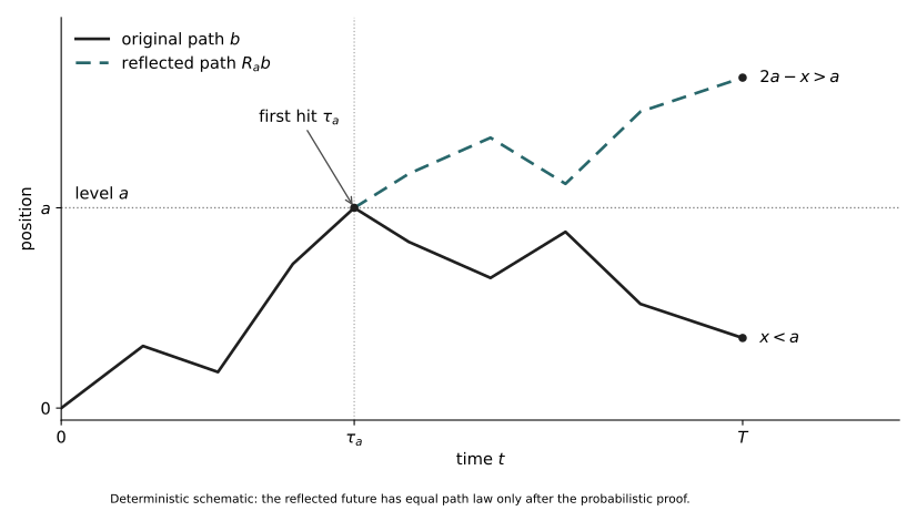
Figure 26.1. A first hit separates a recognizable past from an independent symmetric future. The polygon illustrates the map: endpoint xa. It is not a Brownian sample or a substitute for the strong Markov and measurability proofs. Solid and dashed lines remain distinct in monochrome.
## 26.7 Laws of the maximum and first arrival
Write \(M_t=\max_{s\le t}B_s\). For xt)=2\Phi(a/\sqrt t)-1\sim\sqrt{2/\pi}\,a/\sqrt t\), whose tail integral diverges. A certain arrival can have infinite mean waiting.
We also obtain \(P(\sup_{s\le t}|B_s|>u)\le4e^{-u^2/(2t)}\). The factor four comes from a union bound over positive and negative maxima, not independence. A one-time Gaussian tail has become whole-segment amplitude control.
## 26.8 A certain gain is not a free profit
For a bounded stopping time S, take right-mesh approximations \(S_n\)↓S. The discrete samples \(B_{k2^{-n}}\) form a martingale; Chapter 16’s bounded discrete sampling gives \(EB_{S_n}=0\). If S≤H, all \(S_n\)≤H+1, and reflection makes \(\sup_{u\le H+1}|B_u|\) integrable. Continuity and DCT give \(EB_S=0\), without borrowing an unproved general continuous-time sampling theorem.
\[
EB_{\tau_a\wedge t}=0\quad(t<\infty),\qquad
B_{\tau_a\wedge t}\longrightarrow a\ \text{almost surely},\qquad EB_{\tau_a}=a.
\]
Were the stopped family UI, Chapter 7’s Vitali criterion would pass expectations to the limit, contradicting the display. It is not UI. Fairness is not broken at the hit: increasingly rare, deeply negative terminal paths still carry expectation and cannot be discarded. First-passage tails give concrete meaning to conditions for unbounded sampling.
## 26.9 How strong can continuity be?
Gaussian moments give \(E|B_t-B_s|^p=c_p|t-s|^{p/2}\). Chapter 23’s grid proof gives almost sure γ-Hölder continuity on finite windows for every γ<1/2. Choose p so that γ<1/2−1/p. The original continuous version agrees with that modification at rational times, hence is indistinguishable from it. Intersect over integer windows and countable γ approaching one half.
The path does not fluctuate without constraint: local displacements are bounded by a random constant times \(|t-s|^\gamma\). Can the constant stay finite at γ=1/2? A square-root variance describes a typical increment, not the largest one selected among many locations. First we prove that a finite slope occurs nowhere.
## 26.10 Trap all possible tangent points in a mesh
Fix integers H,M≥1. A finite right derivative at t∈[0,H] would imply \(|B_{t+u}-B_t|\le Mu\) for some δ>0 and all 0
Divide a fixed [a,b] into 2ⁿ equal cells and put \(Q_n=\sum_i(B_{t_i}-B_{t_{i-1}})^2\). Independent Gaussian increments give the following mean and variance. Chebyshev and Borel–Cantelli yield \(Q_n\to b-a\) almost surely.
\[
EQ_n=b-a,\qquad\operatorname{Var}(Q_n)=2(b-a)^2\,2^{-n},\qquad Q_n\longrightarrow b-a.
\]
Sum the absolute displacements along a finite partition, then take the supremum over all partitions: this is total variation, the total travel detectable by arbitrarily fine segmented measurements. A continuous path of finite total variation would satisfy \(Q_n\le\max_i|\Delta B_i|\sum_i|\Delta B_i|\to0\) by uniform continuity, a contradiction. Intersect over rational endpoint intervals; every nondegenerate interval contains one, proving infinite total variation on every such interval.
This proves squared-increment limits along deterministic dyadic partitions. General quadratic variation on random partitions, brackets and Itô integration remain for later chapters. This is not the whole stochastic integration theory. It already shows that failure of first-order length control does not destroy a second-order law.
## 26.12 The extra growth beyond the square root
At each fixed time \(B_t/\sqrt t\) is standard normal. Repeatedly observing one path over longer periods nevertheless finds occasional fluctuations larger than the usual scale. The correction is not another power, but a slowly growing iterated logarithm. First we prove the scalar large-time law, writing \(b(t)=\sqrt{2t\log\log t}\), \(t\ge e^e\).
Fix ε>0 and choose \(1(1+\varepsilon)b(t)\) for some t∈[qⁿ⁻¹,qⁿ], the maximum up to qⁿ exceeds (1+ε)b(qⁿ⁻¹). Reflection and Gaussian tails bound the event by \(2\exp(-c\log\log q^{n-1})\), where \(c=(1+\varepsilon)^2/q>1\). This is summable in n since \(\log\log q^{n-1}=\log((n-1)\log q)\).
Apply Borel–Cantelli and repeat for −B: eventually \(|B_t|\le(1+\varepsilon)b(t)\). A countable intersection over ε↓0 gives limsup≤1 and liminf≥−1. The maximum over a whole block matters; checking B(qⁿ) alone would not exclude crossings between observation times.
## 26.13 Why the lower bound needs separate fresh fluctuations
Now take a large integer q. Increments \(D_n\) on [qⁿ⁻¹,qⁿ] are independent with variance \(q^n(1-1/q)\). For \(0x)\ge c_0x^{-1}e^{-x^2/2}\) gives
\[
\begin{gathered}
D_n=B_{q^n}-B_{q^{n-1}},\\
P(D_n>c\,b(q^n))\ge
C_q(\log n)^{-1/2}n^{-c^2/(1-1/q)}
\quad\text{for all sufficiently large }n.
\end{gathered}
\]
The series diverges, so second Borel–Cantelli gives infinitely many large positive fresh increments. The upper bound controls the old position: \(|B(q^{n-1})|/b(q^n)\le(1+o(1))/\sqrt q\). Thus \(\limsup B_t/b(t)\ge c-1/\sqrt q\). Take countably many integer q increasing to infinity and, for each q, countably many c increasing to √(1−1/q); the lower bound is one. Symmetry handles the negative direction. The normal lower tail follows by integrating the density on [x,x+1/x], not from another limit theorem.
\[
\limsup_{t\to\infty}\frac{B_t}{\sqrt{2t\log\log t}}=1,\qquad
\liminf_{t\to\infty}\frac{B_t}{\sqrt{2t\log\log t}}=-1
\quad\text{almost surely}.
\]
The upper bound uses nearby scales to cover all times; the lower bound uses widely separated scales to reduce the old position. The two choices of q serve different purposes. Conflating them into a parameter varying with n loses the summability and independence arguments.
## 26.14 Turn distant times into a neighborhood of the origin
Time inversion gives a short bridge, but continuity at zero needs verification. Without LIL, Gaussian tails give \(\sum_nP(|B_n|>\varepsilon n)<\infty\) and reflection gives \(\sum_nP(\sup_{u\le1}|B_{n+u}-B_n|>\varepsilon n)<\infty\). Borel–Cantelli and countably many ε↓0 yield \(B_t/t\to0\). Set \(\widehat B_0=0\) and \(\widehat B_t=tB_{1/t}\). It is continuous everywhere, centered Gaussian in finite dimensions, with \(\operatorname{Cov}(\widehat B_s,\widehat B_t)=\min(s,t)\). Chapter 23’s uniqueness on continuous path space makes it standard Brownian. Apply its large-time LIL to obtain
\[
\limsup_{h\downarrow0}
\frac{B_h}{\sqrt{2h\log\log(1/h)}}=1,\qquad
\liminf_{h\downarrow0}
\frac{B_h}{\sqrt{2h\log\log(1/h)}}=-1
\quad\text{almost surely}.
\]
This is the LIL at the fixed origin zero. For each specified deterministic r, \(B_{r+h}-B_r\) is Brownian and obeys the same law; strong Markov also permits any specified almost surely finite stopping time. Do not union exceptional sets over all possible random times. Countably many rational r already prove failure of a one-half-Hölder bound on every nondegenerate interval, because the local iterated-logarithm factor is unbounded.
## 26.15 Search all locations for the largest short increment
A fixed origin and a search for the most violent location are different observations. For T>0 set \(w(B,\delta)=\sup_{\substack{s,t\in[0,T]\\|t-s|\le\delta}}|B_t-B_s|\). Roughly 1/δ candidate locations produce larger extremes than a fixed origin. The exact result is
\[
\lim_{\delta\downarrow0}
\frac{w(B,\delta)}{\sqrt{2\delta\log(1/\delta)}}=1
\quad\text{almost surely}.
\]
A union bound on a coarse grid misses times between mesh points. [T-LIL, Section 2](../foundations/t-lil.md#t-lil-uniform-modulus) uses a δ/m mesh, Gaussian tails for pairs at distance about δ, and reflection for both endpoint errors. Fix m large, then sum over geometric δ. The lower bound uses normal lower tails for about T/δ independent short increments; adjacent scales complete all δ.
The log(1/δ) here does not contradict the log log(1/δ) at a fixed origin. One permits a new favorable location at each scale; the other keeps the same origin. The rules for selecting observations matter as much as one increment’s law.
## 26.16 Can the iterated-logarithm law record an entire shape?
The scalar LIL sees only \(B_T\) and can miss the preceding motion. Compress [0,T] onto [0,1] with the same normalization to obtain continuous functions \(Y_T\). They cannot converge to one curve, as their positive and negative endpoint limits show. We seek all shapes they can repeatedly approach.
\[
\begin{gathered}
Y_T(u)=\frac{B_{Tu}}{\sqrt{2T\log\log T}},\quad0\le u\le1,\quad T\ge e^e,\\
K=\left\{g:g(t)=\int_0^t v(u)\,du,\quad
v\in L^2([0,1]),\quad\int_0^1|v(u)|^2\,du\le1\right\}.
\end{gathered}
\]
The Brownian functional LIL says that almost surely \(\{Y_T:T\ge e^e\}\) is relatively compact in uniform norm and its cluster set as T→∞ is exactly K. Every cluster point must lie in K, and every shape in K must actually occur. Evaluation at one maps K onto [−1,1], with endpoints realized by ±u, so the scalar law is included but genuine path information is added.
Strassen’s 1964 “An Invariance Principle for the Law of the Iterated Logarithm” appeared in Zeitschrift für Wahrscheinlichkeitstheorie und Verwandte Gebiete 3, 211–226, as verified by his publication list. We give a modern independent reconstruction for real Brownian motion, not a proof of the paper’s general invariance principle for independent sums.
## 26.17 Why quadratic energy constrains the shape
Forcing Brownian increments near prescribed Δg on a partition multiplies Gaussian densities and produces \(\sum(\Delta g)^2/\Delta u\). Refinement leaves the squared integral \(\int_0^1|v(u)|^2\,du\) of a velocity in \(g(t)=\int_0^t v(u)\,du\), rather than length. Energy comes directly from the density exponent. Bounded partition energies, a bounded linear functional on steps and L² completeness prove existence and uniqueness of this L² velocity. Absolute continuity of the integral makes g absolutely continuous; no extra singular change is possible. Energy is established directly from increments, without presuming a differentiation theorem for pointwise derivatives.
The full proof is in [T-LIL, Sections 1 and 3–7](../foundations/t-lil.md#t-lil-energy). At \(T_n=q^n\), χ² exponential moments for grid increments and reflection remainders make deviations from K summable; stability under \(g(a\,\cdot)/\sqrt a\) fills all real T. For the lower bound, target rational polygons of energy<1 in disjoint large blocks. Gaussian increment boxes give probabilities roughly \(n^{-I(g)}\), and continuous bridges control the remaining errors. Exponents below one allow second Borel–Cantelli. The old block is controlled to \(O(q^{-1/2})\) before q is increased, not discarded.
Neither Chapter 29’s Schilder theorem nor an unproved path transformation formula is invoked. Smoothness of curves in K does not contradict Brownian roughness: these are macroscopic cluster shapes after expanding the window and compressing fluctuations, not microscopic derivatives of the original curve.
## 26.18 Does symmetry leave half the time above zero?
At every deterministic s>0, P(\(B_s\)>0)=1/2, so positive occupation time \(A_T\) has mean T/2. Mistaking this for an independent coin frequency suggests \(A_T/T\) approaches one half for large T. Neighboring times share a continuous history, however: one long positive excursion occupies many neighboring observations.
\[
A_T=\int_0^T\mathbf1_{\{B_s>0\}}\,ds,\qquad
G_T=\max\{s\le T:B_s=0\},\qquad
\rho_T=\min\{s\le T:B_s=M_T\}.
\]
The other two times record the last return and earliest global maximum. For fixed deterministic T, the three fractions have the same law:
\[
\begin{gathered}
P(U\le x)=\frac2\pi\arcsin\sqrt x,\quad
f_U(x)=\frac1{\pi\sqrt{x(1-x)}}\quad(0
Split at deterministic s. Given \(B_s\)=x≠0, reflection gives probability 2Φ(|x|/√(T−s))−1 of avoiding zero until T. Thus \(G_T\)≤s becomes a comparison of absolute values of two independent standard normals:
\[
P(G_T\le s)=P\!\left(\sqrt{T-s}|Z_2|\le\sqrt{s}|Z_1|\right)
=\frac2\pi\arctan\sqrt{\frac{s}{T-s}}
=\frac2\pi\arcsin\sqrt{\frac{s}{T}}.
\]
The two-dimensional Gaussian angle is uniform, so probability is the angular width of four symmetric sectors. For the maximum time, time reversal and symmetry give past drawdown \(D_s=M_s-B_s\) law \(\sqrt s\,|Z_1|\). The independent future maximum increment has law \(\sqrt{T-s}\,|Z_2|\). The event \(\rho_T\)≤s asks the latter not to exceed the former, producing the same angle.
Distinct maximizers must still be excluded. [T-ARCSINE, Section 3](../foundations/t-arcsine.md#t-arcsine-argmax) inserts rational r between hypothetical maximizers. A future maximum has a continuous law independent of the past and zero probability of tying its maximum exactly. Countably many r give uniqueness for fixed T. The companion treats measurability and the non-stopping nature of \(G_T\) too. Strong Markov is never applied at a last zero or maximizer.
## 26.20 Occupation time requires counting whole excursions
Occupation cannot be reduced to two endpoints. Let R start at zero with independent equiprobable ±1 steps. Count a whole edge as positive when its open interior lies above zero: both 0 to 1 and 1 to 0 count once, while neither 0 to −1 nor −1 to 0 counts. A unit step cannot cross zero without ending there, so this is equivalent to a positive midpoint. Let \(H_{2m}\) count positive edges among the first 2m, and let \(L_{2m}\) be the linear interpolation with time scale 1/(2m) and space scale 1/√(2m). Positive occupation then equals the positive-edge fraction exactly; zero endpoints contribute no time. Cutting at zeros yields completed excursions, each keeping its sign until return, and one unfinished terminal segment. Independent return decompositions and sign symmetry give the exact formula
\[
\begin{gathered}
H_{2m}=\sum_{i=1}^{2m}\mathbf1_{\{R_{i-1}+R_i>0\}},\qquad
L_{2m}\!\left(\frac{i}{2m}\right)=\frac{R_i}{\sqrt{2m}},\\
\int_0^1\mathbf1_{\{L_{2m}(t)>0\}}\,dt=\frac{H_{2m}}{2m},\\
P(H_{2m}=2k)=u_{2k}u_{2m-2k},\qquad
u_{2j}=\frac{\binom{2j}{j}}{4^j},\quad0\le k\le m.
\end{gathered}
\]
Why a product rather than binomial probabilities? The return generating function is \(U(z)=(1-z)^{-1/2}\), with first-return function \(F=1-1/U\). The unfinished segment’s tail generating function is again U. In the bivariate generating function, z counts half the total number of steps m and w counts half the positive-edge count k. A positive excursion of 2j edges contributes \((zw)^j\), while a negative one contributes \(z^j\). \(H_{2m}\) is even because completed excursions and the even-length terminal segment have even lengths. Weighting positive excursions with this convention simplifies the total generating function to U(zw)U(z), giving the formula by coefficients. [T-ARCSINE, Section 4](../foundations/t-arcsine.md#t-arcsine-excursions) proves the decomposition, including the zero-length terminal segment.
Chapter 13’s span-two local CLT gives \(u_{2j}\sim(\pi j)^{-1/2}\), turning interior sums into Riemann sums for the arcsine density. Endpoint mass is bounded by C√ε and cannot be ignored. The polygon’s positive fraction is exactly \(H_{2m}/(2m)\), and Donsker sends the polygon to Brownian motion. Occupation is continuous at paths whose zero set has length zero; Tonelli gives this almost surely for Brownian motion. The continuous mapping theorem genuinely transfers the lattice formula to the Brownian law.
## 26.21 Balanced means and one path’s allocation of time
\[
EU=\frac12,\qquad\operatorname{Var}(U)=\frac18,\qquad
P\!\left(U\notin[1/4,3/4]\right)=\frac23.
\]
Substitute x=sin²θ to compute the values. More importantly, the law of \(A_T/T\) does not change with T, so it cannot converge in probability to one half. The law of large numbers has not failed: independent-sample assumptions never applied to these sign observations. One long excursion can push occupation toward an endpoint; symmetry balances means across paths.
Lévy’s original “Sur certains processus stochastiques homogènes” is in Numdam’s journal archive, catalogued as Compositio Mathematica 7 (1940), 283–339. It is an original-source entry into this path literature. Our grid arguments, excursion generating functions and modern path-space proofs are reconstructions, not claims that this exposition or every intermediate result appeared in one historical source in this form.
## 26.22 Roughness is not absence of structure
The curve that kept revealing corners now has a precise character. It has no finite tangent anywhere and infinite total variation on every interval. Yet its largest short fluctuations have an exact scale, its extremes an iterated-logarithm boundary, and its compressed long-time shapes a quadratic energy constraint. Continuity has not made motion smooth; roughness has not made it mathematically structureless.
A first hit permits restarting; a last return requires future information. Equal positive and negative probabilities at each time do not make one path divide its time equally. None of these distinctions is readable from one Gaussian marginal. Path space, measurable events, stopped information and whole-segment estimates reveal how a distribution unfolds in time.
Brownian motion has a sharp restriction: it does not jump. Rare events produced Poisson laws, and heavy-tailed sums produced stable limits. If increments remain independent and stationary but paths may jump, how can continuous small fluctuations and rare large jumps coexist? Adding vertical lines to a Brownian curve will not answer that. We must understand how one motion splits into independent parts.
**Proofs and original sources.** [T-LIL](../foundations/t-lil.md); [T-ARCSINE](../foundations/t-arcsine.md); [Strassen’s publication list](https://www.math.uni-konstanz.de/~strassen/publ.html) and [the 1964 DOI](https://doi.org/10.1007/BF00534910); [Lévy’s original journal archive](https://numdam.org/item/CM_1940__7__283_0/).
---
# Chapter 27: What If Random Motion Jumps as Well as Diffuses? — Lévy Processes and Lévy–Khintchine Theory
Adding many independent small disturbances need not produce only a continuous rough curve. Consider independent clocks: clock k rings at rate 2ᵏ, and each ring moves the position right by 2⁻ᵏ. Later clocks make smaller but more frequent moves. Every layer contributes expected displacement t over time t.
Adding the layers without alteration gives no finite displacement. Subtract each layer’s expected displacement, however, and the remaining total fluctuation can form an actual random path. The difficulty is not merely allowing tiny jumps: it is deciding how infinitely many of them can coexist.
## 27.1 Every layer is finite; the whole sum need not exist
\[
\begin{gathered}
N_k(t)\sim\operatorname{Poisson}(2^k t),\qquad
J_k(t)=2^{-k}N_k(t),\qquad k\ge1,\\
EJ_k(t)=t,\qquad
E[J_k(t)-t]^2=t\,2^{-k}.
\end{gathered}
\]
These independent Poisson clocks were constructed in Chapter 21 and can coexist on Chapter 8’s countable product space. Infinite total expectation alone would not prove almost sure divergence; the spikes of Chapter 7 warn against that inference. Here a stronger argument is available.
\[
P\{N_k(t)<2^{k-1}t\}
\le\frac{4}{2^k t}\quad(t>0).
\]
Chebyshev and Borel–Cantelli imply that, for each fixed positive t, eventually every layer contributes at least t/2. The uncentered positive series diverges almost surely. The centered variances are summable, so Chapter 12 gives convergence at a fixed time. There is no contradiction: we have changed the summands.
A separate answer at every fixed t is not enough. Such limits need not immediately form one right-continuous path with left limits, and uncountably many probability-one events cannot simply be intersected. This is the same quantifier difficulty encountered in constructing Brownian paths. We must identify admissible jump intensities and turn distributional limits into whole paths.
## 27.2 Preserve the increment structure, not continuity
Brownian and Poisson motion share a useful structure: disjoint time intervals give independent increments, and intervals of equal length give increments with the same distribution. Only Brownian motion is continuous. To study both, preserve the increment structure and require displacements over short times to vanish in probability.
\[
\begin{gathered}
X_0=0,\qquad X_t\in\mathbb R^d,\qquad
X_{t+s}-X_s\overset d=X_t,\\
X_{t_1}-X_{t_0},\ldots,X_{t_m}-X_{t_{m-1}}
\text{ independent}\quad(0=t_0<\cdots
A finite-activity model needs one clock and a mark distribution: rate λ, independent jump sizes with law F. The finite measure λF records both. For the clocks at the beginning, a single total rate is no longer adequate: the total count can be infinite while jumps bounded away from zero still occur at a finite rate.
\[
\nu(B)=\text{mean number per unit time of jumps with size in }B,
\qquad B\subset\mathbb R^d\setminus\{0\}.
\]
For now this is a construction motive, not a fact already proved for every process. We first prescribe a Borel measure and construct clocks; later we recover it from any given Lévy path. Summability of the centered squared fluctuations suggests the condition
\[
\nu(\{0\})=0,\qquad
\int_{\mathbb R^d}(1\wedge\|x\|^2)\,\nu(dx)<\infty .
\]
This is a Lévy measure. Finite mass away from zero prevents infinitely many visible large jumps on a finite interval. Square weighting near zero allows centered fluctuations to be summed in L². Neither absolute first integrability nor finite total mass is required. The opening example places mass 2ᵏ at 2⁻ᵏ: its squared integral is finite, its first integral infinite.
The square condition is not merely a convenient proof assumption. With symmetric small-jump density |x|⁻³ on the line, the truncated characteristic-function modulus has a negative integral exponent. At every nonzero frequency, 1−cos(ux) is bounded below near zero by a constant times u²x², so that exponent tends to minus infinity. The candidate is one at zero and zero elsewhere, hence cannot be a weak probability limit. A deterministic drift changes only phase, not modulus.
## 27.4 Put the clocks for all scales on one space
Partition the nonzero space into the exterior of the unit ball and dyadic annuli. Every piece has finite measure. On each use a Poisson clock of that rate, with independent marks from the normalized restricted measure. Different bands are independent; zero-mass bands are empty. The countable product constructions of Chapters 8 and 10 put these choices on one space.
Each ring produces a pair consisting of time and jump size. Count these points in a random measure N. For nonnegative measurable f, N(f) is the sum of its values over all points, possibly infinite. Countable additivity holds path by path because the measure is a countable sum of Dirac masses.
\[
\begin{gathered}
\mu(ds,dx)=ds\,\nu(dx),\qquad
E e^{-N(f)}=\exp\!\left\{-\int(1-e^{-f})\,d\mu\right\},\\
E N(f)=\int f\,d\mu\quad(f\ge0).
\end{gathered}
\]
On one finite band and one finite time interval, condition on the count. Arrival times are ordered independent uniform points and marks are independent. The conditional Laplace transform is a single-point average raised to that count; averaging the Poisson count gives the first formula. Monotone convergence removes the finite-band restriction. The mean identity follows first for indicators, then simple functions and nonnegative limits.
For disjoint sets of finite intensity, insert a linear combination of their indicators. Factorization of the joint Laplace transform proves both Poisson counts and their independence. N is called a Poisson random measure with intensity μ. The name now abbreviates a constructed object. [The path proof, Section 1](../foundations/t-levy-paths.md#t-levy-prm), extends the argument to all measurable sets.
## 27.5 Compensation does not subtract an infinite constant
Fix a positive cutoff ε. Add jumps larger than ε and at most one, then subtract the expectation on that finite band. Both terms are finite. Only then let ε tend to zero. There is no intermediate expression subtracting an infinite mean from an infinite jump sum.
\[
\begin{gathered}
M^\varepsilon_t=
\int_{(0,t]\times\{\varepsilon<\|x\|\le1\}}
x\,N(ds,dx)-t\int_{\varepsilon<\|x\|\le1}x\,\nu(dx),\\
E M^\varepsilon_t=0,\qquad
E\|M^\delta_t-M^\varepsilon_t\|^2
=t\int_{\delta<\|x\|\le\varepsilon}\|x\|^2\nu(dx),\qquad 0<\delta<\varepsilon\le1.
\end{gathered}
\]
The isometry follows because independent Poisson counts have variance equal to mean. Compute first for simple functions on disjoint finite-intensity sets, then extend using T-LP completeness to deterministic L² functions. The integral here is this deterministic L² extension, not a theory of predictable random integrands.
A finite-cutoff process is a martingale: future counts are independent of the past and compensation makes their conditional mean zero. Apply Chapter 15’s Doob inequality on dyadic time grids, then use right continuity to remove the grid. This gives more than a fixed-time isometry.
\[
\begin{gathered}
v(\varepsilon)=\int_{0<\|x\|\le\varepsilon}\|x\|^2\nu(dx)\downarrow0,\\
E\sup_{t\le T}\|M^\delta_t-M^\varepsilon_t\|^2
\le4T\,v(\varepsilon)\qquad(0<\delta<\varepsilon).
\end{gathered}
\]
## 27.6 How a square estimate constructs an entire path
Choose decreasing cutoffs whose remaining second integrals are at most 2⁻⁴ʲ. On [0,j], the probability that adjacent cutoffs differ in supremum norm by more than 2⁻ʲ is at most 4j2⁻²ʲ, a summable sequence. Borel–Cantelli and telescoping imply uniform convergence on every compact interval on one common probability-one event.
A uniform limit of càdlàg functions is càdlàg: approximate by one sufficiently close cutoff, then use its right continuity and left limits. Fatou extends the estimate to all cutoffs, not just the selected subsequence.
\[
\begin{gathered}
M^{\varepsilon_j}\longrightarrow M
\quad\text{locally uniformly a.s.},\\
E\sup_{t\le T}\|M_t-M^\varepsilon_t\|^2
\le4T\,v(\varepsilon)\to0 .
\end{gathered}
\]
Thus the full cutoff family converges uniformly on compact intervals in probability, abbreviated ucp. Fixed-time L² convergence preserves the martingale property. Factorization of joint increment characteristic functions passes to probability limits, preserving independent stationary increments. Vanishing short-time second moments give stochastic continuity. A common supremum estimate, rather than separate fixed-time answers, has constructed the path.
This is the missing step in the opening example. All its jumps are positive, yet the compensated process is not increasing. Each finite cutoff is deterministic downward motion plus finitely many positive jumps. The limit is defined by the whole sequence of compensated cutoffs, not by an ordinary infinite positive sum minus a finite descending line. It has mean zero and positive variance at each positive time. Increasing paths would make it nonnegative, forcing it to vanish by its zero mean, a contradiction.
## 27.7 Three independent kinds of motion
Add an independent continuous Gaussian motion G with nonnegative covariance matrix A, a deterministic drift, and jumps outside the unit ball. Chapter 23 constructs G from independent Brownian coordinates and a matrix square root. There are only finitely many large jumps on each finite interval, even if their sizes have no mean.
\[
\begin{gathered}
X_t=bt+G_t+
\int_{(0,t]\times\{\|x\|>1\}}x\,N(ds,dx)+M_t,\\
E[G_sG_t^\top]=(s\wedge t)A,\qquad G\perp\!\!\!\perp N .
\end{gathered}
\]
This is already a Lévy process. At a finite cutoff, multiply the independent characteristic functions; compensation subtracts the jump term’s linear part. The Lévy condition dominates the quadratic remainder near zero. Removing the cutoff gives
\[
\begin{gathered}
E e^{i\langle u,X_t\rangle}=e^{t\Psi(u)},\\
\Psi(u)=i\langle b,u\rangle-\frac12u^\top Au+
\int_{\mathbb R^d\setminus\{0\}}
\left(e^{i\langle u,x\rangle}-1-
i\langle u,x\rangle\mathbf1_{\{\|x\|\le1\}}\right)\nu(dx).
\end{gathered}
\]
The subtracted linear term records centering at finite cutoffs; it does not alter jump sizes. The full small-jump first integral may not exist, so it cannot be treated as a finite mean transferred into drift. For a unit-jump Poisson process, the measure is λδ₁ and the Gaussian part is zero. Because the cutoff includes size one, b must equal λ: the compensated component is Nₜ−λt, and adding λt recovers the count. Thus b is not automatically the physical velocity or expectation.
We have proved that parameters construct a process. Lévy–Khintchine theory also asserts the converse: every regular motion with independent stationary increments has precisely this form. Without that converse we would have examples, not a classification.
## 27.8 Why not every law can be a unit-time increment
Divide unit time into n pieces. Its increment must be the sum of n independent identically distributed smaller increments, so its law is infinitely divisible. Chapter 14 proved that limits of infinitesimal independent arrays are infinitely divisible. We now turn that structural fact into explicit unique parameters.
The finite-dimensional Lévy–Khintchine theorem states that a real-vector probability law is infinitely divisible if and only if its characteristic function is the previous exponential at t=1, with a nonnegative symmetric matrix A, a Lévy measure ν and a real vector b. These parameters are unique under a fixed truncation convention. For a Lévy process, multiplying that exponent by time gives every increment law; independence then gives every finite-dimensional distribution.
The path construction proves sufficiency: dividing the parameters by n and adding n independent copies restores the original law. Necessity and uniqueness do not follow by reversing that construction. We develop the two difficult mechanisms: how tightness controls parameters and how to identify them without assuming second moments.
## 27.9 Replace an infinite measure by a finite object
Taking subsequences of ν directly fails because its mass near zero may be infinite. But small jumps enter the exponent only quadratically. Weighting by a function that behaves like a square near zero and is bounded away from it produces a finite measure. A continuous truncation h is convenient for parameter convergence.
\[
\begin{gathered}
h(x)=\frac{x}{1+\|x\|^2},\qquad
w(x)=\frac{\|x\|^2}{1+\|x\|^2},\\
\Psi(u)=i\langle\gamma,u\rangle-\tfrac12u^\top Au+
\int(e^{i\langle u,x\rangle}-1-i\langle u,h(x)\rangle)\nu(dx),\\
b=\gamma+\int\left(x\mathbf1_{\{\|x\|\le1\}}-h(x)\right)\nu(dx).
\end{gathered}
\]
The drift-conversion integral is absolutely convergent: its integrand is cubic near zero and bounded away from zero, where ν has finite mass. Changing truncation does not change jumps, only the compensation assigned to the deterministic linear term.
On the line, place Gaussian variance at the origin to obtain a unique finite canonical measure. The associated integral kernel extends continuously there.
\[
\begin{gathered}
\rho=\sigma^2\delta_0+w\nu,\qquad
\Psi(u)=iu\gamma+\int K_u(x)\rho(dx),\\
K_u(x)=\frac{e^{iux}-1-iux/(1+x^2)}{x^2/(1+x^2)}
\quad(x\ne0),\qquad K_u(0)=-u^2/2.
\end{gathered}
\]
This explains how laws made entirely of jumps can leave a Gaussian limit: weighted mass concentrating at zero contributes the kernel’s quadratic value. Gaussian mass is not a jump of size zero. The atom belongs to the weighted replacement measure, not to ν.
For vectors, retain directions of approach to zero by lifting points into radius-direction space. The second directional moment of the zero layer gives the covariance matrix. Different angular measures may give the same matrix; the angular measure itself is not a unique parameter. [The parameter proof, Section 1](../foundations/t-levy-characteristics.md#t-levy-canonical), supplies the bounded continuous kernel and matrix details.
## 27.10 How tightness controls the parameters
Start with a weakly convergent sequence of represented compound-Poisson-plus-Gaussian laws. Their characteristic functions are uniformly close to one near zero. Taking minus the logarithm of the modulus removes drift and leaves nonnegative terms. Averaging over a small frequency cube turns cosine into a product of coordinate sinc functions.
\[
\begin{gathered}
a(\delta)=\sup_n\sup_{\|u\|_\infty\le\delta}
[-\log|\phi_n(u)|]\longrightarrow0,\\
\frac{\delta^2}{6}\operatorname{tr}A_n+
\int\left[1-\prod_{j=1}^d\operatorname{sinc}(\delta x_j)\right]\nu_n(dx)
\le a(\delta).
\end{gathered}
\]
The kernel bounds δ²‖x‖² below near zero and a positive constant below far away. A fixed small δ bounds total weighted mass; decreasing δ also controls escape to infinity. The finite radius-direction measures are therefore tight, so Chapter 24’s selection applies. Drift cannot escape either: after removing the controlled integral, an unbounded drift admits a frequency tending to zero with phase minus one, contradicting common continuity at zero.
The limiting measure recovers ν at positive radii and A at the zero layer, while drift converges to γ. The continuous kernel transfers parameter limits to characteristic functions. Hence represented laws are closed under weak convergence. No independent jump/Brownian decomposition of a limiting process has been assumed.
To put every infinitely divisible law in that closure, take its nth convolution roots, subtract coordinate medians and then bounded sine means. Local characteristic functions of symmetrizations bound each truncated second moment by O(1/n), making correctly centered roots infinitesimal. Chapter 14’s budget bounds the row sum of those moments. Taylor remainders make the logarithmic difference between the original array and its accompanying compound Poisson law vanish. The original law is a weak limit of represented laws, proving necessity.
This step must not assume convolution roots have globally nonvanishing characteristic functions; the representation will imply that later. [The parameter proof, Sections 3–5](../foundations/t-levy-characteristics.md#t-levy-budget), starts with nonvanishing only near zero and completes centering, error estimates and parameter extraction.
## 27.11 Recover all jumps without second derivatives
Without a second moment, differentiating the exponent twice is invalid. Finite differences remain legitimate: a second difference supplies a nonnegative weight that suppresses small jumps.
\[
\begin{gathered}
-\{\Psi(u+v)+\Psi(u-v)-2\Psi(u)\}=\widehat M_v(u),\\
M_v=(v^\top Av)\delta_0+
2(1-\cos\langle v,x\rangle)\nu(dx).
\end{gathered}
\]
M is finite, so Chapter 14’s Fourier uniqueness applies. Take each coordinate direction and its √2 multiple. Their combined weights are positive at every nonzero point: a nonzero coordinate cannot simultaneously be an integer multiple of 2π and 2π/√2. Add these measures and divide away from zero by that positive weight to recover all of ν.
After removing the jump integral, the real part identifies the entire quadratic form, including off-diagonal entries of A; the imaginary part identifies drift. Two continuous exponents of the same characteristic function differ by integer multiples of 2πi. Connectedness and their zero value at the origin force that difference to vanish. Uniqueness requires no additional moments.
## 27.12 Return to the original path, not just a new model
For a Lévy process already given on a probability space, the unit-time law now has a unique triplet. The ratio of the time-1/n characteristic function to the corresponding exponential is a continuous nth root of unity, equal to one at zero, so is identically one. Independence gives rational times, and stochastic continuity gives all times. Its finite-dimensional distributions match the constructed model.
Matching finite-dimensional laws does not by itself identify an independent Gaussian remainder on the original space. We must read jumps from that path and prove the reading measurable. A càdlàg path has finitely many jumps above a fixed threshold on a compact interval, or an accumulation would violate a one-sided limit. It can also be uniformly approximated by finite step functions.
\[
\begin{gathered}
N_X=\sum_{s>0:\Delta X_s\ne0}\delta_{(s,\Delta X_s)},\\
\sum_i a(t_i)f(X_{t_i}-X_{t_{i-1}})
\longrightarrow \sum_{01\}}x\,N_X(ds,dx)
+\lim_j\int_{(0,t]\times\{\varepsilon_j<\|x\|\le1\}}
x\,[N_X(ds,dx)-ds\,\nu(dx)],\\
C\text{ continuous centered Gaussian},\quad
E[C_sC_t^\top]=(s\wedge t)A,\quad C\perp\!\!\!\perp N_X .
\end{gathered}
\]
The equality holds for all times on one probability-one event. The chosen cutoff subsequence converges locally uniformly; all cutoffs converge ucp. If A is degenerate, the assertion is only that the continuous remainder has covariance A; no extra standard Brownian coordinates are invented on the original space. [The path proof, Sections 4–6](../foundations/t-levy-paths.md#t-levy-original-space), supplies measurability and common-null-set details.
## 27.13 What must converge when laws converge
Poisson approximations may shrink jumps to zero, and a Gaussian limit can arise from those very jumps. The original Gaussian matrices therefore need not separately converge to the final one: unresolved small-jump covariance must be included. Convergence of jump measures away from zero also needs a separate condition excluding escape to infinity.
\[
\begin{gathered}
\mathrm{ID}(\gamma_n,A_n,\nu_n)\Rightarrow\mathrm{ID}(\gamma,A,\nu)
\quad\Longleftrightarrow\\
\gamma_n\to\gamma,\qquad
\nu_n\xrightarrow{v}\nu\text{ on }\mathbb R^d\setminus\{0\},\\
\lim_{R\to\infty}\limsup_n\nu_n(\|x\|>R)=0,\\
\lim_{\varepsilon\downarrow0}\limsup_n
\left\|A_n+\int_{\|x\|\le\varepsilon}xx^\top\nu_n(dx)-A\right\|=0 .
\end{gathered}
\]
All drifts use the same continuous truncation from Section 9. Small radii approach zero through spheres receiving no limiting jump mass. For sufficiency split the exponent into a small ball, compact annulus and remote tail: Taylor remainder is bounded by ε times second mass, vague convergence treats the annulus, and the tail condition treats infinity. Necessity extracts weighted measures along every subsequence and uses uniqueness to identify all limits. [The parameter proof, Section 7](../foundations/t-levy-characteristics.md#t-levy-convergence), records the double-limit order.
On the line this reduces to convergence of γ and weak convergence of finite canonical measures ρ. Removing jumps below ε and adjusting drift approximates the law by compound Poisson plus Gaussian laws. To use only compound Poisson, replace each Gaussian eigendirection by symmetric tiny jumps whose rate times squared size equals its eigenvalue.
\[
\frac{\lambda}{2a^2}\delta_{a e}+
\frac{\lambda}{2a^2}\delta_{-a e}
\quad(a\downarrow0)
\quad\Longrightarrow\quad
\text{Gaussian covariance }\lambda\,ee^\top .
\]
This proves distributional and finite-dimensional time-law approximation. It does not silently assert path-space J₁ convergence from triplet convergence; that additionally requires the path-tightness controls of Chapter 24.
## 27.14 Centering cannot be skipped in array limits
Triangular arrays from Chapter 14 now have a full identification tool. Rows are independent and infinitesimal; terms need not be identically distributed or integrable. Subtract coordinate medians, then bounded sine means. This choice cancels the first-order characteristic expansion while using only expectations of bounded functions.
\[
\begin{gathered}
k=1,\ldots,r_n,\quad r_n<\infty,\qquad \max_{k\le r_n}P(\|Z_{nk}\|>\eta)\to0\quad(\eta>0),\\
Y_{nk}=Z_{nk}-m_{nk},\quad
b_{nk}=E(\sin Y_{nk,1},\ldots,\sin Y_{nk,d}),\quad
W_{nk}=Y_{nk}-b_{nk},\\
d_n=\sum_k(m_{nk}+b_{nk})-c_n,\quad
\nu_n=\sum_k\mathcal L(W_{nk})\big|_{\mathbb R^d\setminus\{0\}},\\
\gamma_n=d_n+\int h\,d\nu_n,\qquad A_n=0 .
\end{gathered}
\]
The centered row sum converges to a specified infinitely divisible law if and only if these triplets satisfy the four conditions above. Replace each correctly centered term by a Poisson number of repetitions. A truncated second-moment budget controls its characteristic-function error, and the total logarithmic remainder is bounded by the largest budget times the total budget, hence vanishes. Conversely recover budget boundedness from the triplet conditions before asserting tightness. [The parameter proof, Sections 5 and 9](../foundations/t-levy-characteristics.md#t-levy-arrays), establishes both directions.
Why not Poissonize raw terms? A row of n deterministic values 1/√n has centered sum identically zero. Raw Poissonization randomizes the count and invents Gaussian variance one. Median centering makes every W zero and retains the correct degenerate limit. Deterministic position and genuine random fluctuation must first be separated.
## 27.15 Infinitely many jumps need not mean infinite variation
Activity and total variation describe different infinities. Finite total ν-mass is equivalent to finitely many jumps on every finite interval, by Poisson counts. With infinite mass, every positive-length rational time interval almost surely contains infinitely many jumps, yet their absolute sizes may still be summable.
\[
\begin{gathered}
X\text{ has finite variation on every compact interval a.s.}\\
\Longleftrightarrow\quad
A=0,\qquad
\int_{0<\|x\|\le1}\|x\|\,\nu(dx)<\infty .
\end{gathered}
\]
Sufficiency is concrete: Campbell’s identity makes the absolute small-jump sum finite, so compensation can be absorbed into finite linear drift. Necessity is more than the slogan that Brownian motion is rough. Infinite absolute small-jump integral makes the absolute jump sum infinite by the Poisson Laplace formula, and the variation of any càdlàg path dominates the sum of its jump norms.
If the Gaussian matrix is nonzero, project onto positive variance. Fix a jump path. If adding Gaussian motion has positive probability of finite variation, use two independent Gaussian copies with that same jump path. Both have finite variation with positive probability, so their difference would be a nonzero scaled Brownian motion of finite variation, contradicting Chapter 26. Fubini over jump paths completes the argument. [The path proof, Section 7](../foundations/t-levy-paths.md#t-levy-variation), supplies the details without invoking general quadratic variation.
\[
\begin{gathered}
d=b-\int_{\|x\|\le1}x\,\nu(dx),\qquad
X_t=dt+\sum_{s\le t}\Delta X_s
\quad\text{in the finite-variation case}.
\end{gathered}
\]
Positive-jump density 1/x on the unit interval has infinite total mass but finite first integral: infinite activity and finite variation. Density 1/x² satisfies the Lévy square condition but not the first-integrability condition, giving infinite variation after compensation. The same visible sign of jumps conceals a different summation mechanism.
## 27.16 No negative jumps does not imply an increasing path
Waiting and cumulative input often require increasing motion. A real Lévy process with nondecreasing paths is a subordinator; here it starts at zero, is not killed and has infinite lifetime. Monotonicity implies finite variation, removing the Gaussian part and non-absolutely-summable small jumps. Jumps must be positive, and the remaining actual linear drift must be nonnegative.
\[
\begin{gathered}
A=0,\quad \nu((-\infty,0))=0,\quad
\int_{(0,1]}x\,\nu(dx)<\infty,\quad
d=b-\int_{(0,1]}x\,\nu(dx)\ge0,\\
E e^{-qX_t}=
\exp\!\left[-t\left(dq+\int_{(0,\infty)}(1-e^{-qx})\nu(dx)\right)\right],
\quad q\ge0.
\end{gathered}
\]
These conditions suffice, since the ordinary positive jump sum constructs increasing paths. To prove the drift sign, split short-time jumps at size ηt. Both the probability of a larger jump and the expectation of the smaller jump sum divided by t vanish. Hence the jump sum divided by t tends to zero in probability, so Xₜ/t tends to d and nonnegativity forces d≥0. Only small-jump first integrability and finite large-jump mass are used.
For example, use density 1/x² only on (0,1), compensate it as above and take b=0. The process has mean zero, variance t and is nondegenerate. Nonnegativity would force a mean-zero variable to vanish, a contradiction. Positive jumps do not eliminate downward compensation: the Lévy measure describes jump directions, while the full path also depends on drift and compensation.
## 27.17 Stable laws become an exhaustive family
Chapter 14 constructed new stable laws through heavy-tail sums, leaving their exhaustive classification open. We can now let uniqueness constrain scaling instead of guessing a characteristic function. Sums of independent copies of a stable law change only location and scale; infinite divisibility supplies a continuous convolution family.
The convergence-of-types lemma prevents arbitrary scale and location changes under the same nondegenerate limit. Extend rational-time stability to real time; multiplication of times makes the scale a continuous multiplicative function, hence a power. Compare temporal and spatial scaling of covariance and jump measure:
\[
\begin{gathered}
a(t)=t^{1/\alpha},\qquad
t\sigma^2=t^{2/\alpha}\sigma^2,\qquad
\nu(rB)=r^{-\alpha}\nu(B),\\
0<\alpha<2:\quad
\nu(dx)=
\bigl(c_+\mathbf1_{\{x>0\}}+c_-\mathbf1_{\{x<0\}}\bigr)
|x|^{-1-\alpha}\,dx,\quad \sigma^2=0,\\
c_\pm\ge0,\quad c_++c_->0;\qquad
\alpha=2:\quad \nu=0,\quad\sigma^2>0.
\end{gathered}
\]
Scale multiplication comes from two operations on the same exponent. Start with the affine expression at time t, then multiply its convolution exponent by s:
\[
st\Psi(u)=\Psi(a(s)a(t)u)
+iu\{a(t)b(s)+s b(t)\}.
\]
This and the affine expression at time st describe one nondegenerate law. Uniqueness of positive scale and location forces a(st)=a(s)a(t). Time continuity turns multiplication into a power law; Gaussian covariance and jump measure must then obey the same scale rather than being chosen separately.
The density is a conclusion. Homogeneity first makes each tail a power; differences on intervals then give the density, and square integrability near zero forces α<2. Nonzero Gaussian variance forces α=2. Removing both leaves deterministic translation, excluded by nondegeneracy. This exhausts nondegenerate real stable laws, rather than treating Cauchy as the whole theory.
Centering at α=1 requires care. Let Δ be the difference of the two density constants. A change of scale moves the truncation boundary and leaves a logarithmic term. It is not an error and cannot be removed by a fixed location shift.
\[
\alpha=1:\qquad Z_1+\cdots+Z_n
\overset d=nZ+n(c_+-c_-)\log n .
\]
Symmetry removes the logarithm; for α≠1 a suitable fixed shift gives strict stability. Density and tail constants differ by a factor α. [The classification and centering proof](../foundations/t-levy-domains.md#t-levy-stable-classification) derives all parameters from convergence of types. Stability is distributional self-similarity under independent addition, not invariance of an individual magnified path.
## 27.18 Read tails back from the limit
Constructing a stable law answers only half the question. Which original variables have sums attracted to it? Sufficiency exhibits a mechanism; necessity rules out other tails producing the same full-sequence limit. A non-Gaussian stable limit requires regular variation of the absolute tail together with balance between its two sides.
\[
\begin{gathered}
F(x)=P(|Z|>x)\text{ regularly varying with index }-\alpha,\quad0<\alpha<2,\\
\frac{P(Z>x)}{F(x)}\to p_+,\qquad
\frac{P(Z<-x)}{F(x)}\to p_-,\qquad p_++p_-=1,\\
nF(a_n)\to C>0,\qquad c_\pm=\alpha C p_\pm,\\
c_n=a_n\{nE h(Z/a_n)-\gamma\}
\quad\Longrightarrow\quad
\frac{S_n-c_n}{a_n}\Rightarrow\mathrm{ID}(\gamma,0,\nu_\alpha).
\end{gathered}
\]
The bounded-function center exists even without a mean. Tail limits identify ν away from zero; regular variation bounds small-jump second mass by a positive power of ε and remote tails by a negative power of R. The triplet criterion then gives sufficiency. Before raw Poissonization one must still control its logarithmic error; a suitable absolute q-moment makes n times the squared single-term characteristic error vanish.
For necessity, do not assume regular variation. Apply the correctly median-centered array criterion to convergent sums, obtaining scaled tail limits at every nonzero threshold. Convergence of types gives adjacent scale ratio one. The first scale crossing any large threshold extends those limits from the scale sequence to all real thresholds. Only then return to raw-term centering and prove the drift condition necessary.
This proves necessary and sufficient conditions for real stable attraction, not merely Chapter 14’s heavy-tail construction. [The domain proof, Sections 4–5](../foundations/t-levy-domains.md#t-levy-stable-domain-sufficient), includes quantile scales, truncation bounds, moving thresholds and centering. Oscillating tails may admit particular subsequential shapes without a full-sequence stable limit.
The exact equality specifying cₙ is a convenient choice; for general centers the necessary and sufficient condition is the following limit.
\[
nE h(Z/a_n)-c_n/a_n\longrightarrow\gamma.
\]
## 27.19 Infinite variance can still leave a Gaussian limit
The division “finite variance means Gaussian, infinite variance means non-Gaussian” is false. The relevant objects are visible large jumps and unresolved small fluctuations at the chosen scale. Some infinite-variance tails are thin enough that large jumps disappear while truncated second mass accumulates into a nonzero atom at zero.
\[
\begin{gathered}
\mu=EZ,\qquad V(x)=E[(Z-\mu)^2\mathbf1_{\{|Z-\mu|\le x\}}],\\
\frac{S_n-c_n}{a_n}\Rightarrow N(\ell,\sigma^2),\quad\sigma^2>0\\
\Longleftrightarrow\
\begin{cases}
E|Z|<\infty,\quad V\text{ slowly varying},\quad a_n\to\infty,\\
nV(a_n)/a_n^2\to\sigma^2,\quad(n\mu-c_n)/a_n\to\ell.
\end{cases}
\end{gathered}
\]
Here Z is nondegenerate, summands are i.i.d. and scales positive; V on the right is defined after integrability is established. Slow variation includes finite positive limiting variance and slowly diverging V. Its tail meaning is that x² times the tail beyond x is negligible relative to V(x): visible large jumps disappear, leaving Gaussian second mass.
Necessity must not assume a mean. First use the independent difference Z−Z′, whose center is zero. Canonical mass concentrating at zero makes its truncated second moment slowly varying. Dyadic tail integrals prove first integrability of the difference; a median tail bound transfers this to Z. Only then subtract the mean and identify its truncated variance as asymptotically half that of the difference. Sufficiency uses the same tail bounds to control jumps, drift and logarithmic errors. [Sections 6–8 of the proof](../foundations/t-levy-domains.md#t-levy-normal-tail) establish both directions.
\[
\begin{gathered}
f(y)=|y|^{-3}\mathbf1_{\{|y|\ge1\}},\qquad
EY=0,\quad EY^2=\infty,\quad V(x)=2\log x\ (x\ge1),\\
a_n=\sqrt{n\log n}\quad(n\ge2),\qquad
\frac{Y_1+\cdots+Y_n}{a_n}\Rightarrow N(0,1).
\end{gathered}
\]
This density is normalized. Square-root time is not the only normalization leading to a Gaussian limit; it is the finite-variance input case. A slowly growing truncated variance changes the scale without leaving a jump measure away from zero. The same parameter-convergence mechanism explains Gaussian and heavy-tail stable limits while preserving their differences.
## 27.20 Why reflection cannot simply survive an overshoot
At first contact Brownian motion is exactly at the target height, giving reflection an exact joining point. Jump motion can overshoot. The overshoot creates additional structure, so Brownian reflection formulas cannot be copied. A discrete random walk makes the distinction transparent.
Fix the signs first: R is the signed displacement of the endpoint from its maximum; D is the usual nonnegative drawdown.
\[
M_n=\max_{0\le j\le n}S_j,\qquad
R_n=S_n-M_n\le0,\qquad D_n=M_n-S_n=-R_n\ge0.
\]
Observe at an independent geometric time N with probabilities (1−z)zⁿ, 00\},\quad
T^-=\inf\{n\ge1:S_n\le0\},\\
F_\pm(z,u)=E[z^{T^\pm}e^{iuS_{T^\pm}};T^\pm<\infty],\\
1-z\phi_Z(u)=\bigl(1-F_+(z,u)\bigr)\bigl(1-F_-(z,u)\bigr).
\end{gathered}
\]
This is the discrete Wiener–Hopf product established here. One side is strict and the other weak because the split uses the first global maximum: ties belong to the later segment. Reversing that segment turns nonpositive prefixes into a weak record minimum at its endpoint. Independence after discrete stopping times gives strict ascending and weak descending ladder renewal series. Their transforms have modulus at most z, so the series converge absolutely. Comparing with the geometric endpoint characteristic function gives the identity.
Making both ladders strict fails for zero increments. [The ladder proof, Section 9](../foundations/t-levy-domains.md#t-levy-wiener-hopf), derives the transform from the unique path split, allowing lattice laws, ties and infinite ladder times. We do not set z to one without justification or claim all continuous-time fluctuation theory. Jumps require height and waiting-time information; continuous reflection is a special geometry.
## 27.21 Historical sources and the proof used here
The representation connects limits of sums of independent random variables with independent-increment motion in time. Lévy’s 1934 paper, “Sur les intégrales dont les éléments sont des variables aléatoires indépendantes,” appeared in the Annali della Scuola Normale Superiore di Pisa and is digitized by Numdam. Khintchine’s 1937 “Zur Theorie der unbeschränkt teilbaren Verteilungsgesetze” addresses infinitely divisible laws; MathNet supplies its official record and original-paper entry.
These are verifiable primary-source entries, not claims that every intermediate lemma or present notation occurs in either original. Our proof is a modern reconstruction using measure theory, tightness, countable coordinates and L² tools. Finite-dimensional parameter compactness, transfer through path jump functionals and domain-of-attraction arguments are organized around this book’s established dependencies. The Poisson random-measure and compensation constructions can also be compared with Winkel’s own Oxford lecture notes.
**Primary sources and proofs.** [Lévy’s 1934 original](https://www.numdam.org/item/ASNSP_1934_2_3_3-4_337_0/); [Khintchine’s 1937 official archive](https://www.mathnet.ru/eng/sm5562); [Winkel’s own lecture notes](https://www.stats.ox.ac.uk/~winkel/ms3b10.pdf); [parameters, uniqueness and arrays](../foundations/t-levy-characteristics.md); [jump paths and original-space decomposition](../foundations/t-levy-paths.md); [stable classification, attraction and ladders](../foundations/t-levy-domains.md).
## 27.22 One increment structure, different kinds of paths
None of the opening clocks has been discarded. We changed how their contributions are combined: visible jumps are added as actual displacements; dense small jumps are compensated at finite cutoffs before a common supremum bound removes the cutoff. Second mass concentrating at zero leaves a continuous Gaussian part; mass remaining away from zero leaves identifiable jumps. Drift records the location convention for this sum.
Brownian and Poisson motion are not unrelated isolated examples. They reveal different components of one structure; stable laws show how tails and scales determine what survives magnification. Continuity, finite activity, finite variation, positive jumps and monotonicity remain distinct properties. A characteristic exponent places them on one verifiable map without erasing their differences.
Our increments still ignore current position. If entering a different region changes the next short segment’s law, one exponent no longer describes the evolution. The assembly based on independent increments must give way to state-dependent transitions, while continuity in time and path regularity still need proof. Having constructed motion from local jump frequencies, we can next investigate how local motion rules act on functions used to observe it.
---
# Chapter 28: Why Does Random Motion Produce Deterministic Equations? — Semigroups, Generators and Resolvents
The next step of a single particle may be unpredictable. Yet if many particles start at the same position, the average of an observable at a later time often has a definite answer. The observable might be a temperature profile, a terminal payoff, or a smooth approximation to a region. Varying the starting position produces a new function: the expected future observation from each starting point.
For a while we follow the changing functions rather than each individual path. Evolution through two time intervals must agree with evolution through the first followed by a fresh start from the new position. Short-time changes should reveal the local motion. Recovering an entire motion from these traces requires much more information than a differential expression alone.
## 28.1 Tomorrow’s Average as a Function Today
Let E be the state space and Pₜ its transition kernels. For a bounded Borel function f define Tₜf. Its argument is the starting position, not time. We choose the observable; the motion transforms every such choice into a new function.
\[
T_t f(x)=\int_E f(y)P_t(x,dy)=E_x f(X_t).
\]
For an indicator this is the probability of reaching an event. General functions preserve linearity, positivity and bounds: averaging cannot make a nonnegative payoff negative or increase its largest possible value. Two distributions with equal integrals against every bounded Borel function are equal. Passing from kernels to observables loses no transition probabilities.
For a countable chain this is matrix multiplication on a column vector. For Brownian motion it is Gaussian convolution. For Chapter 27’s jump motion it is still averaging, with a displacement law accommodating continuous fluctuations and jumps. We need a language in which these are instances of the same operation.
## 28.2 Joining Time Intervals Means Composing Operators
\[
P_{s+t}(x,B)=\int_E P_t(y,B)P_s(x,dy),\qquad T_{s+t}=T_sT_t,\qquad T_0=I.
\]
Chapter 17’s Chapman–Kolmogorov equation becomes the semigroup law. First average over the last t units conditional on the intermediate state, then average over the first s units. Fubini proves the identity for nonnegative functions; decomposition proves it for bounded functions. Time homogeneity matters: calendar-dependent rules require a two-parameter evolution, not dependence solely on elapsed time.
The algebraic law does not yet say whether short times produce small changes. An instantaneous resampling rule may satisfy it while failing to approach the initial state. We must choose a function space in which a short time really gives a small change.
## 28.3 Why Not Use Every Bounded Function?
Even deterministic translation is not norm-continuous on discontinuous observables. Translating a half-line indicator by any positive distance changes its value by one somewhere. The motion is not discontinuous; the instrument has a sharp edge.
\[
T_t f(x)=f(x+t),\qquad f=\mathbf1_{[0,\infty)},\qquad \|T_t f-f\|_\infty=1\quad(t>0).
\]
Throughout E is a locally compact Polish space. We use the real Banach space C₀(E): continuous functions whose absolute value is at least any positive ε only on a compact set, with the supremum norm. Observations fade at infinity, and nonzero absolute extrema are attained. If E is compact this is C(E). Uniform Cauchy sequences have uniform continuous limits still vanishing at infinity, proving completeness.
A C₀-Feller semigroup satisfies the semigroup law, is positive and contractive, preserves C₀, and has the following strong continuity. “Strong” refers to norm convergence for each fixed function, not operator-norm convergence uniformly over the unit ball.
\[
\lim_{t\downarrow0}\|T_t f-f\|_\infty=0\qquad(f\in C_0(E)).
\]
Positivity and contraction allow mass below one, so our operator convention initially permits killing. We separately call the semigroup conservative if the corresponding kernels have mass one from every starting point. Operator norm one cannot replace this pointwise requirement.
## 28.4 From Lévy Displacements to a Feller Semigroup
Let Tₜf(x) be the expected value of f at x plus a Lévy displacement. Independent stationary increments give the semigroup law. A Euclidean C₀ function is uniformly continuous: use uniform continuity on a large compact neighborhood and small function values outside. This yields a modulus estimate.
\[
\|T_t f-f\|_\infty\le\omega_f(\delta)+2\|f\|_\infty P(|X_t|>\delta).
\]
Let time tend to zero and then δ tend to zero to get strong continuity. For fixed time, restrict the displacement to a large ball with small probability outside. As the starting position goes to infinity, f is small at all endpoints inside that ball. Thus Tₜf stays in C₀. Only Chapter 27’s process construction and stochastic continuity are used, not its attraction-domain or Wiener–Hopf classifications.
## 28.5 Why the Short-Time Rate Needs a Domain
Translation leaves a first derivative; Brownian averaging leaves a second derivative. Continuous functions need not have either. Requiring a generator on all of C₀ would exclude the very motions we want to understand. We must record both the rule and the observables where it makes sense.
\[
D(A)=\left\{f\in C_0(E):\lim_{h\downarrow0}\frac{T_hf-f}{h}\text{ exists in }C_0(E)\right\},\qquad Af=\lim_{h\downarrow0}\frac{T_hf-f}{h}.
\]
This is a norm limit: errors become small uniformly over starting points, and the result remains continuous and vanishes at infinity. For a domain element, the semigroup law transports the derivative at zero to every time, and left and right difference quotients give the following identity. The Riemann construction and fundamental theorem for continuous Banach-valued integrals are proved in [T-OPERATORS](../foundations/t-operators.md#t-operators-integrals).
\[
T_t f-f=\int_0^tT_sAf\,ds,\qquad \frac{d}{dt}T_tf=AT_tf=T_tAf\quad(f\in D(A)).
\]
This is a precise meaning of random averages producing deterministic equations. Domain elements give classical norm-differentiable solutions. Other initial functions receive their continuous evolution from the semigroup, and cannot simply be differentiated without proof.
## 28.6 How a Partial Operator Controls the Whole Space
The domain contains more than a few smooth toy functions. Average any f over a short time interval and shift the interval to compute its generator.
\[
f_t=\frac1t\int_0^tT_sf\,ds\in D(A),\qquad Af_t=\frac{T_tf-f}{t},\qquad f_t\longrightarrow f.
\]
Thus the domain is dense. If fₙ and Afₙ converge in norm to f and g, pass to the limit in the integral identity, divide by t, and let t decrease to zero. Then f belongs to the domain and Af=g. This closedness prevents incompatible limits of observations and rates. Closed does not mean bounded: fixed-height functions can have increasingly large slopes. We need a bounded inverse operation, not an artificial bound on A itself.
## 28.7 A Random Inspection Time and Discounted Occupation
Let the instrument read f at an independent exponential clock. At rate λ its expected reading is λRλf. Removing λ gives accumulated observations with later payoffs exponentially discounted.
\[
R_\lambda f=\int_0^\infty e^{-\lambda t}T_tf\,dt,\qquad \|R_\lambda\|\le\lambda^{-1},\qquad\lambda>0.
\]
This is the resolvent. It first appears as a Laplace transform in time, not an arbitrary algebraic trick. Contraction controls the infinite tail and positivity is retained. Apply Tₕ, change variables, separate the initial short interval and take a difference quotient to get the first inverse relation. Integrating the derivative of discounted Tₜf for a domain element gives the second; exponential decay removes the endpoint at infinity.
\[
(\lambda-A)R_\lambda f=f\quad(f\in C_0),\qquad R_\lambda(\lambda-A)f=f\quad(f\in D(A)).
\]
The resolvent range is exactly the generator domain. An evolution difficult to differentiate is recorded by a bounded inverse on every continuous observable. The exponential clock turns time evolution into a linear equation.
## 28.8 Consistency Across Discount Scales
\[
R_\lambda-R_\mu=(\mu-\lambda)R_\lambda R_\mu,\qquad R_\lambda R_\mu=R_\mu R_\lambda,\qquad \lambda R_\lambda f\longrightarrow f\quad(\lambda\to\infty).
\]
Subtracting the inverse relations gives the first two identities. The last says that increasingly fast inspection sees the initial state: split the integral near zero and into an exponential tail, using strong continuity and contraction. See [T-OPERATORS](../foundations/t-operators.md#t-operators-resolvent) for the full calculation. The entire family is constrained; inverses cannot be chosen independently for each λ.
Smaller λ lengthens the observation time but does not ensure equilibrium. Uniform rotation on a circle oscillates forever, although discounted averages converge to the circular average. For a unit circle one has the following identity.
\[
\lambda R_\lambda f(x)=\frac{\lambda}{1-e^{-\lambda}}\int_0^1e^{-\lambda s}f(x+s)\,ds\longrightarrow\int_0^1 f(s)\,ds\quad(\lambda\downarrow0).
\]
If Tₜf already converges in norm to g, substitution u=λt and dominated convergence give λRλf→g. Rotation disproves the converse. At λ=0 undiscounted occupation may even be infinite: for one-dimensional Brownian motion and a nonzero nonnegative compactly supported observable, the Gaussian density has a lower bound of order t⁻¹ᐟ² on a fixed compact interval.
## 28.9 Reconstructing a Semigroup from Local Rules
Reverse direction and start with a densely defined linear operator A, without assuming a process. Probabilistic averaging requires Af(x)≤0 whenever f attains a nonnegative global maximum at x. This positive maximum principle is the local trace of contraction, but it does not guarantee solvability of the rate equation.
The probabilistic Hille–Yosida theorem proved here says: if A maps a dense linear domain of real C₀ into C₀, satisfies the positive maximum principle, and λ₀−A has dense range for some positive λ₀, then A is closable and its closure generates a unique positive strongly continuous contraction semigroup. Mass loss is initially allowed; conservativity is separate.
Simply citing a generation theorem would hide the central difficulty. Applying the maximum principle at positive and negative extrema gives estimates controlling the inverse norm and positivity. The companion proves closability and surjectivity for every positive λ step by step; we now exhibit the construction itself.
\[
\lambda\|f\|_\infty\le\|(\lambda-A)f\|_\infty,\qquad\lambda\|f^-\|_\infty\le\|((\lambda-A)f)^-\|_\infty.
\]
## 28.10 Yosida Approximation: Random Inspections Replace an Unbounded Rate
\[
A_\lambda=\lambda(\lambda R_\lambda-I),\qquad S_\lambda(t)=e^{tA_\lambda}=e^{-\lambda t}\sum_{k=0}^\infty\frac{(\lambda t)^k}{k!}(\lambda R_\lambda)^k.
\]
Each inspection updates by λRλ, and its count is Poisson, making the approximation positive and contractive automatically. More frequent inspections make Aλf approach Af on the domain. Commuting resolvents give commuting bounded approximations; differentiation and integration yield a direct Cauchy bound.
\[
\sup_{0\le t\le T}\|S_\lambda(t)f-S_\mu(t)f\|_\infty\le T\|(A_\lambda-A_\mu)f\|_\infty\longrightarrow0\quad(f\in D(A)).
\]
In this construction first replace the closable candidate by its closure; A henceforth denotes that closure. Take the limit on the dense domain, then extend by contraction. Uniform convergence on compact time intervals preserves the semigroup law and strong continuity. Surjectivity of λ−A finally rules out an extra domain in the limiting generator, identifying it exactly with the closure of A. [T-OPERATORS](../foundations/t-operators.md#t-operators-generation) proves this and uniqueness without stochastic integration or a preexisting path.
## 28.11 Which Test Functions Really Determine the Generator?
Dense tests can identify measures without identifying unbounded operators. Af must be approximated alongside f. A subspace D₀ dense in the following graph norm is called a core. Equivalently its range under λ−A is dense for one positive λ.
\[
\|f\|_A=\|f\|_\infty+\|Af\|_\infty,\qquad D_0\text{ is a core}\iff\overline{(\lambda-A)D_0}=C_0(E).
\]
To prove it, approximate (λ−A)f and apply the bounded inverse Rλ, obtaining both approximations; the converse follows from graph-norm continuity. The maximum principle alone is insufficient. On (0,1), Af=f′ on compactly supported smooth functions has its range annihilated by the following nonzero continuous functional. The range is not dense: boundary information is missing.
\[
\int_0^1e^{-\lambda x}(\lambda f(x)-f^{\prime}(x))\,dx=0\qquad(f\in C_c^\infty(0,1)).
\]
## 28.12 One Second-Order Expression, Two Processes
On [0,∞), Brownian motion may stay at zero after reaching it, or reflect there. Both have interior rate one half of the second derivative. Starting at zero, one stays put while the other spreads out. Zero is a state; stopping there differs from killing by departure. With Gaussian density gₜ of variance t and standard normal distribution function Φ, reflection gives two semigroups.
\[
\begin{aligned}T_t^r f(x)&=\int_0^\infty[g_t(y-x)+g_t(y+x)]f(y)\,dy,\\T_t^a f(x)&=\int_0^\infty[g_t(y-x)-g_t(y+x)]f(y)\,dy+2\Phi(-x/\sqrt t)f(0).\end{aligned}
\]
Absorption retaining zero gives Af(0)=0, requiring f″(0)=0 for the continuous second-derivative expression. Reflection requires f′(0)=0. These are not domains assigned by intuition: the companion computes the full resolvent ranges through Green kernels to prove these equalities, with one-sided derivatives at zero.
\[
\begin{aligned}D(A_a)&=\{f\in C_0([0,\infty))\cap C^2([0,\infty)):f^{\prime\prime}\in C_0,\ f^{\prime\prime}(0)=0\},\\D(A_r)&=\{f\in C_0([0,\infty))\cap C^2([0,\infty)):f^{\prime\prime}\in C_0,\ f^{\prime}(0)=0\}.\end{aligned}
\]
Smooth compactly supported functions constant near zero give identical operators and form a dense class in C₀, but are a core for neither. [T-FELLER-EXAMPLES](../foundations/t-feller-examples.md#t-feller-boundary-domains) shows how graph norms retain boundary information. A formal differential expression can omit the entire fate at a boundary.
## 28.13 The Lévy Triplet as a Rule on Functions
For smooth compactly supported f, Chapter 27’s Gaussian fluctuation, drift and compensated jumps give the following generator. Q is the Gaussian covariance matrix and b uses unit-ball truncation.
\[
Af(x)=b\cdot\nabla f(x)+\frac12\operatorname{tr}(Q\nabla^2 f(x))+\int_{\mathbb R^d\setminus\{0\}}[f(x+y)-f(x)-\mathbf1_{\{|y|\le1\}}y\cdot\nabla f(x)]\,\nu(dy).
\]
Subtracting the first-order term makes the small-jump remainder quadratic. Without it absolute integrability can fail, just as ordinary small-jump summation failed. The proof truncates small jumps, differentiates a finite Poisson series and Gaussian Taylor expansion, then controls semigroup differences by the coupled L² maximal bound and generator differences by the Taylor remainder. Passing the integral identity to the limit proves genuine domain membership. See [T-FELLER-EXAMPLES](../foundations/t-feller-examples.md#t-feller-levy-generator). Complex exponentials outside C₀ are not domain elements, and smooth tests are not called a core without graph approximation.
## 28.14 Recovering Probability Kernels from Operators
Operator generation has not constructed a random experiment. For fixed t and x, the bounded positive functional f↦Tₜf(x) must be shown to integrate a measure. We need only Riesz representation for bounded positive C₀ functionals on locally compact Polish spaces. The companion builds discrete measures from finite partitions on compact spaces, uses Chapter 24’s tightness theorem, and then one-point compactification. No future general random-measure theory is assumed.
Increasing nonnegative C₀ approximations to open-set indicators make the resulting subprobability measures measurable in the starting point. A monotone class extends this to Borel sets. The semigroup identity and uniqueness of representation give Chapman–Kolmogorov, recovering consistent transition probabilities.
Conservativity is separate. On compact E it is equivalent to one belonging to the domain with A1=0; on noncompact E, one usually is not in C₀. A sufficient condition is a domain sequence 0≤fₙ≤1 tending pointwise to one with generator norms tending to zero. The integral identity makes Tₜfₙ−fₙ uniformly small; bounded convergence gives mass one. In contrast A=−I gives exponential killing. Chapter 22’s pure birth process with rates 2ⁿ also shows that formally zero row sums do not exclude explosion; a formal A1=0 cannot replace conservativity.
## 28.15 Finite-Dimensional Rules Still Need Regular Paths
Assume conservativity from here. Chapter 8 gives a coordinate process with these finite-dimensional laws, but Chapter 23 shows that finite-dimensional rules cannot exclude pathological modifications at random times. We still owe E-valued càdlàg paths on one event of probability one. Resolvents provide controllable observations: for nonnegative f and λ>0, the process \(e^{-\lambda t}R_\lambda f(X_t)\) is a supermartingale, since waiting removes a nonnegative part of occupation.
\[
e^{-\lambda s}T_sR_\lambda f=\int_s^\infty e^{-\lambda r}T_rf\,dr\le R_\lambda f.
\]
Use a countable dense nonnegative class and integer λ. Chapter 15’s crossing inequalities on finite rational grids exclude infinite oscillations, giving rational side limits at every real time simultaneously. One-point compactification supplies cluster points and separating observables make them unique. A cluster point might still be infinity: no loss at each deterministic time does not exclude escape at a random time.
## 28.16 How Conservativity Controls a Whole Path Segment
Take increasing compactly supported cutoffs χₘ tending to one and put gₘ=αRαχₘ. Conservativity makes 0≤gₘ≤1 increase pointwise to one. One minus discounted gₘ(Xq) is a nonnegative submartingale; the finite-grid maximal inequality bounds escape from a superlevel set.
\[
P_\pi\!\left(\inf_{q\in\mathbb Q\cap[0,T]}g_m(X_q)<\delta\right)\le\frac{1-e^{-\alpha T}E_\pi g_m(X_T)}{1-\delta},\qquad0<\delta<1.
\]
Choose α small and then m large to make the bound arbitrarily small. Yet {gₘ≥δ} is compact inside E. Choose compact sets with error tending to zero and take finite unions to make them increasing. Almost every rational path on all of [0,T] is contained in one of them, so every side limit remains in E.
Define the new process by rational right limits. A compatible metric built from the countable observations, with finite-coordinate and series-tail control, proves càdlàg paths. Strong continuity makes observation increments converge in second mean, proving equality with the old process almost surely at fixed times. See [T-FELLER-PATHS](../foundations/t-feller-paths.md#t-feller-regularization). The scope is conservative C₀-Feller semigroups on locally compact Polish spaces, not arbitrary weak-Feller kernels.
## 28.17 Can We Restart at a Time Chosen by the Path?
Fix an initial law π and complete the natural filtration. Markov recursion for continuous cylinder functions and Chapter 15’s reverse conditional-expectation limit prove right continuity of this completed filtration; details are in the companion. Completion is for π, not a single implicit completion for all initial laws. For a bounded stopping time use upward dyadic approximation. An event A in the stopped σ-algebra allows deterministic Markov on each grid slice.
\[
\tau_n=2^{-n}\lceil2^n\tau\rceil\downarrow\tau,\qquad E_\pi[\mathbf1_A f(X_{\tau_n+s})]=E_\pi[\mathbf1_A T_sf(X_{\tau_n})].
\]
First take f in C₀. The left side uses right-continuous paths; the right additionally needs continuity of Tₛf, precisely where the Feller property matters. After dominated convergence, constants and a monotone class extend to bounded Borel functions. Localize unbounded τ by τ∧m, stating the result only on finite τ.
\[
E_\pi[f(X_{\tau+s})\mid\mathcal F_\tau]=T_sf(X_\tau)\quad\text{on }\{\tau<\infty\}.
\]
Recursion handles several future times and a rational-coordinate π–λ argument handles the future path. The companion also proves stopped-state measurability and open-set entrance times. Closed-set entrance cannot simply be identified with limits of open-neighborhood entrances: a jump path’s left limit alone may touch the closed set.
## 28.18 Generator Error as a Fair Game
For a domain element f, subtract the time accumulation of Af from the actual change. The remainder is not zero pathwise, but is a conditionally fair fluctuation.
\[
M_t=f(X_t)-f(X_0)-\int_0^tAf(X_s)\,ds.
\]
The Markov property gives the conditional mean of f(Xₜ), and conditional Fubini gives that of the integral. The semigroup identity cancels them, so M is a càdlàg martingale. Bounded Af justifies the integrals. For bounded stopping τ, expand on finite grids into martingale increments with past-measurable indicators, then use right continuity and a deterministic bound. This gives Dynkin’s formula without importing later general continuous-time sampling.
\[
E_xf(X_\tau)-f(x)=E_x\int_0^\tau Af(X_s)\,ds.
\]
A stopping time with finite expectation is handled by τ∧n, since the integral is bounded by its length times the norm of Af. Without such a condition the undiscounted version cannot be used arbitrarily. See the grid proof in [T-FELLER-PATHS](../foundations/t-feller-paths.md#t-feller-dynkin).
## 28.19 What Remains of the Resolvent After Stopping?
Put u=Rλf, so (λ−A)u=f. The semigroup identity directly proves a discounted martingale; summation by parts against the finite-variation exponential is another route requiring no stochastic integral. Every stopping time τ, including infinite τ, then satisfies the following formula.
\[
R_\lambda f(x)=E_x\!\left[\int_0^\tau e^{-\lambda s}f(X_s)\,ds+\mathbf1_{\{\tau<\infty\}}e^{-\lambda\tau}R_\lambda f(X_\tau)\right].
\]
Prove this first for τ∧n. An integrable exponential tail dominates the integral, and discount removes the terminal term on infinite τ. The resolvent splits into observations earned before stopping and the remaining observation restarted from the stopped state. As both a linear-equation solution and an expected path occupation, it gives boundary problems a probabilistic meaning.
## 28.20 Exactly What Does a Generator Determine?
A closed densely defined operator with its domain and generation conditions uniquely determines a strongly continuous semigroup. Positivity gives subprobability kernels, conservativity gives probability kernels, local compactness and Feller structure give an E-valued càdlàg realization, and grid approximation gives strong Markov. Each step adds different content.
“Determining a process” means determining finite-dimensional laws for every initial law and the law on the coordinate σ-algebra of càdlàg paths. It does not assert pathwise uniqueness on an arbitrary prescribed probability space. Nor does a formal operator on a few tests automatically meet generation conditions. Boundary behavior and explosion expose false uniqueness claims caused by merging these levels.
Can a process be identified merely by requiring observations minus generator accumulations to be fair? This leads later to the martingale problem. Our existence and uniqueness proof has not assumed it.
## 28.21 The Deterministic Record Left by Random Paths
A particle may jump, or move continuously and nowhere differentiably. Its average action on continuous payoffs nevertheless forms a continuous operator semigroup. The generator does not erase randomness: it records short-time averages, while the domain retains which observations reliably read that rate, especially at boundaries.
The resolvent joins local readings to an entire span of time. Exponential-clock averaging, discounted occupation and the inverse generator are different roles of the same operation. Their constraints reconstruct kernels from operators and paths from kernels, rather than relying on a formal analogy between motion and equations.
This volume asks what discrete records retain and what shared control yields a genuine path. Random geometry now also has deterministic readings. If attention turns from typical paths to exceptionally unlikely deviations of whole trajectories, weak-convergence scales are still too coarse. With path space established, the new difficulty is measuring motions that become harder to observe without becoming impossible.
### Sources and Proof Scope
Mathematical comparisons use Engel and Nagel’s [A Short Course on Operator Semigroups](https://www.math.uni-tuebingen.de/de/forschung/agfa/members/a_short_course_on_operator_semigroups-1.pdf) and Schilling’s author notes [An Introduction to Lévy and Feller Processes](https://arxiv.org/abs/1603.00251). This is a modern reconstruction for the book’s problem sequence, not a reconstruction of the original discovery order. General growth semigroups, non-locally-compact states, general martingale problems and arbitrary nonconservative path theories are outside the proved scope.
---
# Chapter 29: When Small Probabilities Become Exponentially Small — Large Deviations
A fair coin tossed n times lands heads every time with probability 2⁻ⁿ. This outcome is n/2 away from the expected number of heads. The central limit theorem identifies a width of order √n around the mean. It does not say whether its bell curve can be extended all the way to “every toss is heads.”
Extrapolating the local Gaussian quadratic exponent to that location gives a cost n/2, whereas the exact coin calculation gives n log 2. Both probabilities are small and exponentially decaying, but their ratio still grows or shrinks exponentially. For exceptionally rare events, “roughly small” is not nearly enough.
## 29.1 The Bell Curve Never Promised to Reach That Far
Let Bᵢ be iid Bernoulli variables with 01−p it is empty. The CLT controls fixed finite intervals for the standardized variable, whereas a fixed deviation in the interior range sends the threshold to infinity. Weak convergence does not control these escaping sets.
\[
\frac{\sqrt n(\overline B_n-p)}{\sqrt{p(1-p)}}\Rightarrow N(0,1),\qquad \{\overline B_n\ge p+a\}=\left\{\frac{\sqrt n(\overline B_n-p)}{\sqrt{p(1-p)}}\ge\frac{a\sqrt n}{\sqrt{p(1-p)}}\right\}.
\]
This is not a small defect in CLT accuracy: the scale of the question has changed. We fix a macroscopic deviation and increase the number of trials, asking the probability cost of sustaining it. Begin with the case where counting gives the cost directly.
## 29.2 The Cost of an Atypical Collection of Coins
Take 0
Independent costs multiply and logarithms add them. Repeating an experiment at n-fold scale often multiplies its logarithmic cost by n. We therefore divide the logarithm of probability by a speed aₙ tending to infinity. At this scale a finite collection of alternative routes is governed by the largest probability.
\[
\max_{i\le r}b_{n,i}\le\sum_{i=1}^r b_{n,i}\le r\max_{i\le r}b_{n,i},\qquad a_n^{-1}\log r\longrightarrow0.
\]
We cannot demand the same limit for every event. A continuous law assigns zero probability to a point, yet its neighborhoods may have finite exponential cost; a boundary can also cut through attainable records. The large deviation principle preserves this distinction through open lower bounds and closed upper bounds.
Let Zₙ take values in a metric space S. A lower-semicontinuous I:S→[0,∞] is a rate function. The variables satisfy an LDP at speed aₙ with rate I if every open G and closed F satisfy the following bounds, with log 0=−∞ and the infimum over the empty set equal to infinity.
\[
-\inf_G I\le\liminf_n\frac1{a_n}\log P(Z_n\in G),\qquad \limsup_n\frac1{a_n}\log P(Z_n\in F)\le-\inf_F I.
\]
For a Borel event A, sandwich between its interior and closure. If their infimal costs agree, a logarithmic limit follows. I is not a density: it records neighborhood costs at a specified scale. Changing the scale or topology can change the answer.
## 29.4 Why a Rate Function Should Be Good
When minimizing the cost of a deviation, candidate records might escape to infinity without realizing their limiting cost. Compact finite-cost sublevel sets prevent that escape. Such a rate function is called good.
\[
\{x:I(x)\le L\}\text{ is compact for every finite }L.
\]
Goodness concerns the geometry of cost, not ordinary tightness of random variables. It gives convergent subsequences of bounded-cost approximate minimizers; lower semicontinuity retains their limiting cost. Contraction, closed-set neighborhood limits and path energy will all use this mechanism.
## 29.5 Ordinary Tightness Misses Exponential Escape
Let Zₙ equal zero with probability 1−1/n and n with probability 1/n. It converges in probability to zero and its laws are tight. Yet outside any fixed compact set the probability is still eventually 1/n. Its logarithm divided by n tends to zero, not an arbitrarily large negative number.
Exponential tightness requires, for each L>0, a compact Kᴸ whose escape probability has upper logarithmic rate at most −L. Ordinary tightness asks for small probability. Here it must be small fast enough at the scale under study.
\[
\limsup_n a_n^{-1}\log P(Z_n\notin K^L)\le-L.
\]
This is the missing control from local to global. Given open lower and compact upper bounds, split closed F into F∩Kᴸ and escape from Kᴸ. The finite-sum logarithmic rule bounds the result by max{−inf_F I,−L}; let L increase to get the closed upper bound. Ordinary tightness cannot supply this step.
## 29.6 How Costs Change When the Observation Changes
Given costs for full records, read only a continuous statistic Φ. Many records can yield the same value. The cost of a reading y should be the least cost among records producing it. This is the contraction principle.
\[
J(y)=\inf\{I(x):\Phi(x)=y\}.
\]
Assume I is good. On a nonempty fiber of finite infimal cost, a minimizing sequence has a convergent subsequence in an I-sublevel set. Continuity retains the fiber and lower semicontinuity retains the cost, so the minimum is attained. A J-sublevel is exactly the continuous image of an I-sublevel and is compact. Open and closed preimages and the original LDP prove both bounds for Φ(Zₙ).
Continuity matters. If Zₙ is normal with variance 1/n, let Φ(x)=1 exactly at zero and zero elsewhere. Then Φ(Zₙ) is always zero. The formal fiber formula would give cost I(0)=0 at y=1, contradicting the open lower bound. A discontinuity at one point can invalidate a formal contraction.
## 29.7 Making Rare Samples Typical Under Another Law
When coin frequencies depart from p toward q, they are typical if observed under a coin whose head probability is q. We can use a law of large numbers under that law and then restore the original record weights. For random vectors, multiply by an exponential linear weight and divide by its normalizer.
\[
\Lambda(\theta)=\log\int e^{\langle\theta,x\rangle}\mu(dx),\qquad \mu_\theta(dx)=e^{\langle\theta,x\rangle-\Lambda(\theta)}\mu(dx)\quad(\Lambda(\theta)<\infty).
\]
For a finite sample the old and new weights differ by an exponential determined by the sample mean. If the tilted mean is the target x, its neighborhood has probability tending to one under the tilted law, at cost θ·x−Λ(θ). Chernoff gives the same expression from above. Tilting is where upper and lower bounds meet, not merely a computational trick.
Cramér published his work on deviations of sums in 1938. Our finite-dimensional and entropy method is a modern reconstruction, not a claim to reproduce his original proof order. The important difficulty is that not every x is a tilted mean. Proving only parameter-matched points does not prove the general theorem.
## 29.8 The Information Cost of Replacing a Distribution
To avoid being confined to one exponential family, allow any replacement law ν whose mean is near the target. If ν is absolutely continuous with respect to μ, its density ρ records each sample’s reweighting. For typical ν-samples, the mean log weight tends to the following quantity; n independent observations pay n times that cost.
\[
H(\nu\mid\mu)=\int\rho\log\rho\,d\mu=\int\log\rho\,d\nu\quad(\nu\ll\mu),\qquad H(\nu\mid\mu)=\infty\quad(\nu\not\ll\mu).
\]
Use 0 log 0=0. There is no infinity-minus-infinity ambiguity: r|log r|≤1/e for 0
Let Xᵢ be iid vectors in Rᵈ with law μ, and assume Λ is finite on an open neighborhood of zero. Their sample means satisfy an LDP at speed n with the following good rate function. Laws supported on a proper affine subspace are included; no nonsingular covariance is required.
\[
I(x)=\Lambda^*(x)=\sup_{\theta\in\mathbb R^d}\{\langle\theta,x\rangle-\Lambda(\theta)\}.
\]
First prove the upper bound. For fixed x and finite Λ(θ), a sample mean in its δ-ball has scalar product at least θ·x−|θ|δ. Exponential Markov and independence give the following estimate. Choose θ approaching I(x) and use finite covers for compact upper bounds. If I(x) is infinite, choose arbitrarily large finite targets.
\[
P\{\overline X_n\in B(x,\delta)\}\le\exp\{-n[\langle\theta,x\rangle-|\theta|\delta-\Lambda(\theta)]\}.
\]
Exponential moments near zero extend the result to noncompact closed sets. Choose positive η with finite Λ at ±ηeⱼ; coordinate Chernoff bounds control escape from a large cube. The same tests bound the sublevel sets of I. As a supremum of continuous affine functions I is lower-semicontinuous. Thus goodness and exponential tightness are established separately.
\[
P(\|\overline X_n\|_\infty>R)\le2d\,e^{-n(\eta R-C)},\qquad I(x)\ge\eta\|x\|_\infty-C,\quad C=\max_{j,\pm}\Lambda(\pm\eta e_j).
\]
## 29.10 The Lower Bound Must Survive Missing Tilt Parameters
Take ν with finite first moment and finite entropy, whose mean x belongs to open G. A law of large numbers places its sample mean in G. Its log density is integrable, so another law places the mean log weight near H. Restore μ-weights only on this typical event to obtain the open lower bound.
\[
\mu^{\otimes n}(\overline X_n\in G)\ge e^{-n(H(\nu\mid\mu)+\delta)}\nu^{\otimes n}\!\left(\overline X_n\in G,\ \frac1n\sum_{i=1}^n\log\rho(X_i)\le H(\nu\mid\mu)+\delta\right).
\]
The probability in parentheses tends to one. The relation is an inequality, not always equality: ν may vanish on sets with positive μ-mass. This is a finite-product change of measure, not a density between infinite sample laws, where such a density often does not exist.
\[
J(x)=\inf\{H(\nu\mid\mu):\int|y|\nu(dy)<\infty,\ \int y\nu(dy)=x\}.
\]
The open lower bound is therefore −inf_G J. We still must identify it with I. Mixtures and convexity of r log r make J convex, but not necessarily closed. The entropy inequality bounds its convex conjugate by Λ. Conversely truncate an exponential tilt to a large ball: samples are bounded, entropy is finite, and the normalizer increases to the moment generating function. This proves that the conjugate of J is exactly Λ.
Nearest-point separation of finite-dimensional closed convex epigraphs then proves that the lower-semicontinuous closure of J equals the conjugate of Λ; no unproved variational principle is invoked. Closing J does not change its infimum on an open set, since nearby means eventually remain in that set. [T-LDP](../foundations/t-ldp.md#t-ldp-cramer-lower) gives the separation, truncation and limit order in full. The general lower bound follows, including missing-tilt boundary and degenerate cases.
## 29.11 A Gaussian Limit Is Not the Required Tail Condition
For a normal law Λ is linear plus quadratic, giving a quadratic cost about the mean. For a Poisson law with parameter λ>0 the cost is x log(x/λ)−x+λ for x≥0, infinity for negative x, and λ at zero by continuity. These are deviations of means with different global costs. The full exponential reading of the law, not merely its variance, determines the answer.
Finite variance cannot replace exponential moments. Take a nonnegative Pareto variable with tail x⁻ᵝ for x≥1 and β>2. It satisfies a finite-variance CLT, yet one variable exceeding na suffices to push the sample mean above a. For a above the true mean, the following probability has no strictly positive cost at speed n.
\[
P(\overline X_n>a)\ge P(X_1>na)=(na)^{-\beta},\qquad \lim_{n\to\infty}\frac1n\log P(\overline X_n>a)=0.
\]
The displayed lower bound and probability at most one give the equality. A single large jump realizes the deviation, making this exponential scale lose discrimination. If all Xᵢ equal one nondegenerate Y, their mean stays Y; identical marginal laws cannot replace independence either.
Even with exponential moments, ordinary tilting need not reach every target. For density proportional to e⁻ˣ(1+x)⁻³ on x≥0, the parameter reaches only θ=1. The endpoint tilt has density 2(1+x)⁻³ and mean one; larger targets lie outside the tilted-mean range. The preceding closure argument preserves the lower bound at these points rather than excluding them from the theorem.
## 29.12 When the Entire Empirical Distribution Deviates
A mean compresses many records into one number. Samples with the same mean may concentrate near the center or at two extremes. To ask whether data resemble another distribution, retain their empirical measure, assigning mass 1/n to each observation, instead of inventing a separate theorem for every statistic.
\[
L_n=\frac1n\sum_{i=1}^n\delta_{X_i}\in\mathcal P(E).
\]
Let E be Polish and μ any common law. Use Chapter 24’s weak topology, reading integrals of bounded continuous functions; a basic neighborhood constrains finitely many readings. Sanov’s theorem says Lₙ satisfies an LDP at speed n with good rate H(·|μ). No moment generating function or finite state space is required.
Finite alphabets suggest the answer through multinomial counting: each type has log probability equal to minus n times its discrete relative entropy, up to logarithmic error. Infinite spaces do not provide finitely many types to count. We must organize all continuously readable local evidence into entropy.
## 29.13 Why Entropy Is the Strongest Exponential Test
\[
H(\nu\mid\mu)=\sup_{f\in C_b(E)}\left\{\int f\,d\nu-\log\int e^f\,d\mu\right\}.
\]
Each f supplies testable evidence: samples resembling ν should have f-average near νf. Exponential Markov measures the rarity of that evidence by its exponential mean under μ. Taking every test says that entropy is not an added penalty, but the strongest exponential cost supplied jointly by bounded continuous evidence.
The identity needs proof. First allow bounded Borel tests. Re-normalizing μ by eᶠ and using nonnegative entropy bounds each test by H. Truncating logρ to [−M,M] and letting M increase gives the reverse inequality. If ν charges a μ-null set, M times its indicator makes the supremum infinite. Finally approximate bounded Borel functions in L¹(μ+ν) by equally bounded continuous functions. The exponential is Lipschitz on a fixed bounded interval, allowing replacement by C_b. [T-SANOV](../foundations/t-sanov.md#t-sanov-entropy) proves the approximations and their limit order.
Each test is weakly continuous, so H is lower-semicontinuous. Finite entropy also limits mass placed in regions rare under μ. For 0b. This persists in a weak neighborhood, while independence gives the exact exponential moment below. Exponential Markov bounds its probability by e⁻ⁿᵇ; finite compact covers give the compact upper bound.
\[
E_\mu e^{nL_nf}=\left(\int e^f\,d\mu\right)^n.
\]
For finite-entropy ν in open G, observe ν-samples. Laws of large numbers for finitely many continuous readings place Lₙ in G; a law for logρ controls the cost of returning to μ. The same finite-product inequality as for means gives −H. Minimize over ν for the open lower bound. Full support is not required; this does not make the two infinite sample measures equivalent.
The closed upper bound remains. Ordinary tightness of empirical measures is not enough. Given L>0, choose δⱼ=2⁻ʲ and compact Kⱼ with extremely small μ-tails: set θⱼ=(L+j+1)/δⱼ and μ(Kⱼᶜ)≤e⁻ᶿʲ. Requiring every tail mass to be at most δⱼ defines a weakly closed uniformly tight, hence compact, set of measures. Chernoff for the Bernoulli tail counts bounds failure of constraint j by e⁻ⁿ⁽ᴸ⁺ʲ⁾; the infinite union is still at most e⁻ⁿᴸ. The calculation covers even nδⱼ<1.
Intersect the closed set with this compact set and discard the exponentially negligible remainder to complete Sanov. [T-SANOV](../foundations/t-sanov.md#t-sanov-proof) gives parameter choices, weak closedness and infinite sums. The 1957 original paper must be distinguished from this modern Polish-space organization.
## 29.15 An Empirical Law Does Not Make Every Statistic Continuous
Sanov retains more information than a mean, but weak contraction cannot directly give deviations of arbitrary unbounded means. The laws νₘ=(1−1/m)δ₀+(1/m)δₘ converge weakly to δ₀ while their means remain one. A little mass escapes to infinity, vanishing from bounded continuous readings while carrying the entire mean.
Cramér’s exponential moments control such tail contributions. We proved the mean and empirical-measure theorems separately instead of hiding a discontinuous statistic inside contraction. For a bounded continuous payoff f, contraction is legitimate: the cost of its mean reading y is the least entropy among laws with νf=y.
## 29.16 Every Finite Record Can Behave Normally While Paths Escape
Now replace an empirical record by a whole motion. Finite-dimensional exponential estimates are still insufficient. On [0,T] let hₙ be a deterministic triangular spike of height one centered at T/(n+1), supported within distance T/[3(n+1)] of its center and zero outside. At each fixed t its value is eventually zero. Every finite-dimensional record therefore has a trivial LDP charging zero cost only to the zero vector.
Yet the paths have no uniformly convergent subsequence, and their point masses are not exponentially tight. The set {hₙ:n≥1} is closed and separated from the zero path, with probability always one. A full path upper bound based on the zero-path rate would incorrectly be minus infinity. No finite-dimensional calculation is wrong; together they miss increasingly narrow oscillations.
Chapter 24 required shared oscillation control for weak path limits. At a large-deviation scale its failure probability must also be exponentially small enough. Simply carrying over a “small probability” from ordinary tightness is insufficient.
## 29.17 Shrinking Noise and Reading an Atypical Brownian Path
Fix T>0 and a standard d-dimensional Brownian motion B. Study √ε B as ε decreases to zero. Typical paths approach zero uniformly, but reaching a neighborhood of a nonzero continuous curve is not impossible. We use the uniform norm on continuous paths starting at zero, writing this space as \(\mathcal C_T\), distinct from Chapter 28’s C₀ of functions vanishing at infinity.
\[
\mathcal C_T=\{h\in C([0,T];\mathbb R^d):h(0)=0\},\qquad X^\varepsilon=\sqrt\varepsilon B,\qquad a_\varepsilon=\varepsilon^{-1}.
\]
Schilder’s theorem gives total squared velocity as the good rate. A continuous path without a square-integrable velocity representation has infinite cost. Absolute continuity is essential: a continuous path can concentrate variation on a Lebesgue-null set, a hidden motion that finite energy cannot permit.
\[
I_T(h)=\begin{cases}\displaystyle\frac12\int_0^T|g(s)|^2\,ds,&h(t)=\displaystyle\int_0^tg(s)\,ds,\ g\in L^2([0,T];\mathbb R^d),\\\infty,&\text{otherwise}.\end{cases}
\]
This is not a path theorem obtained merely by guessing from a Gaussian squared exponent. We must calculate energy on grids, prove that the grids retain every finite-cost path, and control motion missed between observations.
## 29.18 From Gaussian Increments to Polygonal Path Costs
Take m equal intervals of length Δ=T/m and let Πₘ interpolate grid values linearly. The independent increment density has the following exponent. Its prefactor, a power of ε, disappears after taking logarithms and multiplying by ε. Each squared displacement is divided by its elapsed time, not simply summed without time weights.
\[
E_m(h)=\frac12\sum_{j=1}^m\frac{|h(j\Delta)-h((j-1)\Delta)|^2}{\Delta}.
\]
A density lower bound on an open ball gives the open lower bound; volume times the maximal density gives compact upper bounds. An exponential moment of a Gaussian square controls distant points and completes noncompact closed bounds. The continuous finite-dimensional polygonal embedding gives the full LDP of ΠₘXε: energy Eₘ on that polygonal subspace and infinity off it. [T-SCHILDER](../foundations/t-schilder.md#t-schilder-grid) supplies this density proof rather than substituting a CLT or ordinary weak convergence.
## 29.19 Why Grid Energies Force a Square-Integrable Velocity
Use nested dyadic grids m=2ᵏ. Cauchy–Schwarz shows that refinement cannot decrease energy. Let vₖ be the piecewise constant velocity of Π₂ᵏh. Its finer counterpart averages to the coarse velocity in each coarse cell, giving the orthogonal difference identity.
\[
\|v_\ell-v_k\|_2^2=\|v_\ell\|_2^2-\|v_k\|_2^2\quad(\ell\ge k),\qquad\|v_k\|_2^2=2E_{2^k}(h).
\]
Bounded grid energies make the right side tend to zero as k and ℓ increase, so the velocities are Cauchy in L². Completeness established before Chapter 15 gives a limit g. The uniform integration error is at most √T times the L² error. Since the polygons also converge uniformly to h, we obtain h(t)=∫g. This genuinely excludes continuous but non-absolutely-continuous paths.
Conversely, if h=∫g with g in L², Jensen for cell averages bounds the energies by its squared integral. The same Cauchy argument gives a velocity limit whose integral to every t is h. Measure uniqueness identifies it with g almost everywhere. This gives an exact identification, not merely a one-sided estimate.
\[
I_T(h)=\sup_{k\ge0}E_{2^k}(h).
\]
Each grid energy is continuous, so I is lower-semicontinuous. I≤L also gives the common oscillation bound below; Arzelà–Ascoli makes its sublevel compact. Finite cost permits neither unbounded motion nor fixed-height spikes of arbitrarily small width.
\[
|h(t)-h(s)|\le\sqrt{2L}\,|t-s|^{1/2},\qquad\|h\|_\infty\le\sqrt{2LT}\quad(I_T(h)\le L).
\]
## 29.20 The Missed Motion Must Be Rarer Than the Target Event
On each interval the Brownian path’s difference from its chord is at most twice its maximal increment from the left endpoint. If a Euclidean d-dimensional error exceeds δ, some coordinate exceeds δ/√d. Chapter 26’s reflection tail and union bounds over coordinates and intervals give the following estimate, without assuming independent bridges.
\[
P\{\|X^\varepsilon-\Pi_mX^\varepsilon\|_\infty>\delta\}\le4dm\exp\!\left\{-\frac{\delta^2m}{8dT\varepsilon}\right\}.
\]
Let ε decrease first and then m increase. The error event can be assigned arbitrarily large exponential cost: this is an exponentially good approximation. For one fixed m the error is not automatically superexponentially small. The order of limits matters, and a fixed-grid approximation is not automatically exponentially equivalent to the path.
Ordinary approximation only makes the error probability tend to zero; it may remain much larger than the target e⁻ᶜ⁄ᵋ. We need a rarer error before subtracting it from the probability that a polygon approaches the target. This is real additional work beyond weak path convergence.
## 29.21 Turning All Grid Costs into a Path Theorem
First establish path exponential tightness, not as a synonym for ordinary tightness. Given L>0 choose δⱼ→0 and increasingly fine dyadic mⱼ so that δⱼ²mⱼ/(8dT), with the prefactor 4dmⱼ accounted for, is sufficiently large. Require a uniform path bound and distance at most δⱼ from its polygon for every j. Bounded polygons on each fixed grid form a compact set. Errors δⱼ→0 give total boundedness; the constraints are closed and the space complete, hence compact.
The preceding estimate and the Brownian maximal tail make the infinite union of constraint failures decay at any prescribed exponential rate. Its prefactors grow with j and must be absorbed when choosing mⱼ, not ignored term by term in an infinite sum. The companion supplies explicit parameters.
For compact K, membership of Xε in K implies its projection lies in ΠₘK. The finite-dimensional upper bound gives −inf_K Eₘ. Dyadic energies increase, and compactness allows refinement to commute with taking the infimum: otherwise a cluster point of low-energy candidates would contradict the limiting energy bound. This gives −inf_K I. Exponential tightness extends it to every closed set.
For finite-energy h in open G choose a ball contained in G. Select a sufficiently fine but fixed grid so Πₘh is close to h and the failure cost strictly exceeds I(h). The polygonal neighborhood costs at most Eₘ(h)≤I(h). Subtracting the exponentially smaller error retains that lower bound. Optimize over h to complete Schilder, not only its finite-dimensional part.
[T-SCHILDER](../foundations/t-schilder.md#t-schilder-full) writes out the exponential compact sets, limit order and subtraction lemma in full. No Girsanov theorem, stochastic integral or unproved path variational principle is used.
## 29.22 Which Errors Are Negligible at the Exponential Scale?
Variables Zₙ and Yₙ on the same space are exponentially equivalent at speed aₙ if, for every positive δ, their distance exceeds δ with probability decaying faster than every e⁻ᴸᵃⁿ. This is a precise condition for changing an approximation without changing its LDP.
\[
\limsup_n a_n^{-1}\log P\{d(Z_n,Y_n)>\delta\}=-\infty\qquad(\delta>0).
\]
If Zₙ has an LDP with good rate I, Yₙ has the same LDP. Bound a closed F by the probability that Zₙ lies in its closed δ-neighborhood plus the error, then let δ decrease. Goodness makes the neighborhood infima converge to the infimum on F: bounded-cost candidates have a convergent subsequence whose vanishing distance forces its limit into F. The neighborhoods themselves need not be compact.
For the open lower bound use a ball inside G and subtract the superexponentially small error via the preceding subtraction lemma. See [T-LDP](../foundations/t-ldp.md#t-ldp-equivalence) for the proof. In Schilder’s construction a grid m(ε) tending to infinity gives exponential equivalence by the explicit tail bound. Our fixed-grid proof first established the path LDP independently, without circular reasoning.
## 29.23 When Probabilities Become Exponential Integrals
If records cost I but an observer rewards them by exp(aₙΦ), reward and cost subtract on the logarithmic scale. An LDP yields the following Laplace formula, initially restricted precisely to bounded continuous Φ.
\[
\lim_n a_n^{-1}\log E e^{a_n\Phi(Z_n)}=\sup_x\{\Phi(x)-I(x)\}.
\]
For the lower bound use a small open neighborhood where Φ≥Φ(x)−δ and the LDP lower bound. For the upper bound split its bounded range into finitely many bins of width δ. Bound each contribution by the exponential at the upper endpoint times P(Φ≥the lower endpoint), a closed event. The finite-sum rule gives at most sup(Φ−I)+δ. Let δ decrease. This proves the variational formula rather than assuming it.
An unbounded Φ needs additional exponential tail control. Just as an unbounded mean cannot be contracted weakly without further work, exponential rewards can let tiny masses far away dominate the answer.
## 29.24 How Squared Energy Answers a Concrete Crossing Question
For one-dimensional Brownian small noise, require reaching a positive height b before T. If a finite-energy path reaches b at s≤T, Cauchy–Schwarz gives energy at least b²/(2s), hence b²/(2T). The straight line h(t)=bt/T attains the infimum. The maximum is a continuous uniform-topology reading; the open event maximum>b and closed event maximum≥b have the same infimal cost: take \(h_\eta(t)=(b+\eta)t/T\) and let η decrease to zero to approach that cost from the open side.
\[
\lim_{\varepsilon\downarrow0}\varepsilon\log P\left\{\sup_{t\le T}\sqrt\varepsilon B_t\ge b\right\}=-\frac{b^2}{2T}.
\]
Chapter 26’s reflection formula gives the same exponent, but energy now reveals a transferable mechanism: uniform velocity minimizes squared cost for a prescribed displacement in finite time. This does not assert pathwise convergence of conditioned trajectories to a line, or identify probability cost with physical dissipation. Such claims require additional models and results.
It also explains why differentiating every sample path would be wrong. Brownian paths remain rough and almost surely outside the finite-energy class at every ε. Finite-energy paths describe the costs of rare neighborhoods; Brownian samples have not suddenly acquired differentiability.
## 29.25 The Scales of the Typical and the Rare
All-heads records do not violate the law of large numbers, and distant deviations do not refute the CLT. They demand a different scale. Logarithms turn products of independent weights into additive costs; minimization asks which alternative records can realize the same deviation.
Exponential tilting and convex closure identify the cost of means. Relative entropy prices changing an entire empirical law. Squared energy survives refinement of continuous Gaussian records. These are not three unrelated formulas: each seeks an observation under which rare records become analyzable, while accounting faithfully for the reweighting cost.
The common structure does not erase the distinctions. Finite-dimensional laws do not replace paths, weak tightness does not replace exponential tightness, small errors need not be exponentially negligible, and finite variance does not replace the needed tail conditions. Only after constructing a path can its geometry support such extreme questions.
If we move beyond observing completed paths and act while motion unfolds, using only information already seen, function spaces and distributions no longer suffice. Which information is currently available and which quantities can be chosen before the next noise arrives become mathematical data. A different necessity remains: not only to describe a motion, but to specify precisely what can be known when within it.
### Sources and Scope
Cramér’s 1938 paper can be checked through its [attributed translation and original publication information](https://arxiv.org/abs/1802.05988). See [Sanov’s 1957 journal archive](https://www.mathnet.ru/eng/sm/v84/i1/p11) and [the institutional archive for Schilder’s 1966 paper](https://research.ibm.com/publications/some-asymptotic-formulas-for-wiener-integrals), which retains the title and original-paper link. Modern proofs were compared with [Varadhan’s author notes](https://math.nyu.edu/faculty/varadhan/LDP/Spring2010.3.pdf). Our narrative and proof organization are independent modern reconstructions, not claims that all three originals used today’s Polish-space, convex-closure and grid arguments in this form.
The proved scope is finite-dimensional iid Cramér under exponential moments near zero, Sanov in the Polish weak topology, Schilder for standard d-dimensional Brownian motion on a finite time interval with the uniform topology, and contraction, exponential equivalence and the bounded continuous Laplace formula under the stated assumptions. Deviations of general dynamics, Freidlin–Wentzell for small-noise SDEs and unbounded exponential rewards do not follow automatically and require their own prerequisites.
---
# Epilogue to Volume IV: Bringing an Entire Motion into Mathematics
A microscope leaves records of positions; motion takes place between them. Writing down the joint distribution at every finite collection of times tells us how to compare those records. It does not by itself justify a continuous curve between them. A random spike can evade every observation time fixed in advance; increasingly narrow oscillations can hide between increasingly fine sampling points. To make an entire motion a mathematical object, we must control precisely what finite observations do not directly retain.
Continuity is therefore not a line added when drawing a picture. Once common increment estimates ensure a continuous modification, records on a countable dense set of times can determine the whole continuous path. We preserve the probabilistic information supplied by finite-dimensional distributions and prove that it can unfold consistently in a measurable path space. Path existence requires both parts.
Constructing a path and proving that a sequence of random paths approaches it remain different tasks. The latter also requires control over the whole family: increasingly violent motion must not escape into increasingly short gaps in time. Tightness turns this requirement into common conditions we can check. We first retain most of the probability on path sets subject to uniform control, then use finite observations to identify possible limits. Only then does the Gaussian limit of a random walk become a conclusion about an entire motion rather than a succession of position distributions.
Even “approaching” has more than one meaning. Moving the time of a jump slightly can leave a uniform distance as large as the whole jump height. A small adjustment of time can instead retain the same jump while disregarding a small timing error. This choice cannot erase arbitrary oscillations. A topology specifies which perturbations are small and determines which observations remain stable under passage to the limit. It is part of the limiting assertion.
Once the whole path comes into view, the distance between continuity and smoothness becomes apparent. A Brownian path has no velocity in the ordinary sense, yet its oscillation scales and quadratic variation can be identified rigorously. With jumps allowed, infinitely many small jumps may sometimes be summed directly; in other cases we must first subtract their mean contribution and control the fluctuations left over. Finite-time distribution calculations remain useful, but they must work together with these path structures.
Another route seems to run in the opposite direction: rather than follow one motion, average a function of its future position. Random transitions become a deterministic evolution of operators, and their short-time changes give a generator. Yet the same interior differential formula can accommodate different boundary behavior. Only after specifying the domain, the semigroup conditions, and the requirements for path realization can a local formula determine a random motion in the reverse direction. Averaging has not removed randomness; it has expressed its consistently transmitted structure as an equation.
Exceptionally rare paths require a further change of scale. Ordinary weak convergence describes the overall limit of path distributions, but that limit alone cannot distinguish how small vanishing probabilities are. Large deviations compare path neighborhoods whose probabilities vanish and identify their different exponential costs. For small-noise Brownian motion, squared energy measures the cost of a deviation route. It does not mean that typical Brownian paths suddenly acquire an integrable velocity. Ordinary and exponential tightness, weak approximation and control of errors on an exponential scale, answer different questions.
An entire motion can now enter probability theory: we can establish its existence, compare its shape, study its averages, and measure the cost of its departures from typical behavior. But accumulating a quantity along such a rough path still cannot simply follow the rules for smooth curves. What information may be used as we accumulate, and what will the small fluctuations and jumps leave behind? These questions bring path geometry together with information evolving in time. After understanding the shape of a motion, we still need to learn how to calculate along it.
---
# Volume V · The Calculus of Random Motion
How can calculus respect both rough paths and the order of information?
To calculate an accumulated quantity along a fixed curve, we usually divide time into small pieces and multiply a value on each piece by the curve's increment. If the curve is sufficiently regular, choosing left endpoints, right endpoints, or slightly different partition points does not change the final answer. Brownian motion removes this familiar guarantee: its paths are continuous, yet the absolute amounts of their small changes have no finite sum. Refining a partition does not by itself make the error disappear.
Another distinction has nothing to do with smoothness. Consider deciding how many units of an asset to hold before its next price change, as opposed to filling in the holding for that interval after observing the change. Both records can be written along the same path. Both may use only data that have appeared by a particular time. They nevertheless describe different experiments. The first rule faces an unknown change; the second can exploit the change that has just occurred. On a discrete time grid, before and after remain distinct. When the grid disappears and an event arrives at a single instant, this distinction needs a mathematical expression of its own.
Rebuilding integration therefore requires more than a better choice of partitions. We must specify when the rule being integrated has already been determined, which changes form an accumulation identifiable in advance, and which fluctuations still have no bias given current information. The same path equipped with different information structures may have different decompositions. Temporal order is mathematical data of the model here, not an unconditional claim about causation in the world.
Roughness is not merely an obstacle to exclude. The quantity left by squared increments under refinement suggests that an ordinary first-order approximation may miss a contribution that really persists. Repeated crossings near a position suggest that ordinary residence time may not reveal all the geometry. Calculation must follow these emerging structures, rather than substitute random paths into formulas for smooth curves. Compensation, stochastic integration, and new rules for changes of variables will have different jobs; construction and proof must establish how they fit together.
This route will also test equations in the reverse direction. Specifying local rules of change does not make the symbols on the page an existing motion. Changing a boundary, a noise, or the permitted information can change the answer. A reliable stochastic calculus should explain how to accumulate and transform quantities, and under what conditions those calculations actually describe a random path.
This volume begins with a distinction that is small but indispensable: what we already know while something is happening. Only after drawing that boundary can calculation along random motion respect both the roughness of paths and the order in which information unfolds.
---
# Chapter 30: What Does It Mean to Know Before It Happens?
An arrival occurs. A recorder draws a vertical mark; someone else sees the mark and then writes at the same position, “I was waiting for an arrival here.” The timestamps agree perfectly. That agreement does not mean the second person anticipated the arrival.
In a finite sequence of bets, a time step separates choosing a stake from revealing its outcome. Continuous time has no smallest step. A rule can use only information available by each present time and still exploit a jump that has just occurred at that very time. Before calculating accumulations along random paths, we must distinguish these two meanings of “already known.”
## 30.1 Seeing a Jump Does Not Let Us Backdate a Choice
Take a Poisson process N of rate λ>0 with its complete right-continuous natural filtration. Chapter 21 proves independent arrivals on disjoint time intervals and the martingale property of Mₜ=Nₜ−λt. No new integration theory is needed yet. On a finite interval N has finitely many jumps and λt has finite variation, so ordinary pathwise Stieltjes integrals against them are available.
Choose a bounded ξ using Fₛ before acting on (s,t]. Conditional averaging says that the compensated gain over this interval has no bias. The same remains true for a finite sum of such choices.
\[ E\!\left[\xi\bigl(N_t-N_s-\lambda(t-s)\bigr)\right]=0,\qquad \xi\in L^\infty(\mathcal F_s). \]
Now use Hₜ=ΔNₜ: take value one exactly when an arrival occurs and zero otherwise. H is adapted and can be read from the record up to t. It takes value one at every jump but zero almost everywhere for length measure. Consequently,
\[ \int_{(0,K]}H_t\,dN_t-\lambda\int_0^K H_t\,dt=N_K,\qquad E N_K=\lambda K. \]
The calculation is correct. The mistake would be to identify “readable afterward” with “chosen beforehand.” Adaptedness alone cannot justify extending the earlier conditional-mean identity to every such rule. We need control over the boundary between the two times.
## 30.2 An Event Also Needs a Time Coordinate
A random variable needs measurability on Ω. A process H is a function on Ω×[0,K]; checking Hₜ separately loses their common measurable structure. We need to distinguish two kinds of rules on the product space, rather than choose an unrelated exceptional null set at every time.
The optional σ-algebra O is generated by all càdlàg adapted real processes. “Optional” does not mean permission to use arbitrary future information. It describes information readable from a path as currently displayed. Arrival counts, right-continuous prices, and first-arrival indicators belong here.
The other class places a choice before the interval on which it acts: use an Fₛ-measurable ξ on (s,t], and F₀ at the initial time. The σ-algebra generated by these rectangles is denoted P and called the predictable σ-algebra. It is equivalently generated by all left-continuous adapted processes.
\[ \mathcal P=\sigma\!\left(\{B\times\{0\}:B\in\mathcal F_0\},\ \{B\times(s,t]:B\in\mathcal F_s,\ 0\le s0, hence predictable. Xₜ can include a newly observed jump. Fixed-time tests may miss the distinction completely: ΔNₜ=0 almost surely at every deterministic t, but \(\Delta N_T=1\) at the first arrival T.
Thus “at every fixed t it almost surely equals something known beforehand” cannot replace predictability of the whole process. Chapter 23 distinguished modifications from indistinguishable versions. Here the same issue of incompatible exceptional sets directly affects whether a rule may be used in an accumulation.
Information just before a random time T is precisely the σ-algebra below. It retains F₀ and statements of the form “B was observed at s and T had not yet arrived.” If H is predictable, \(H_T\) on {T<∞} is \(\mathcal F_{T-}\)-measurable. This follows from the rectangular generators and the monotone class theorem, without requiring T to be announceable.
\[ \mathcal F_{T-}=\sigma\!\left(\mathcal F_0,\ B\cap\{st. Right continuity controls information obtained by approaching from the right; completeness lets us remove a common exceptional set. These are conditions on the filtration, not a promise of continuity for every adapted process.
Under the usual conditions, the closed martingale E[Y|Fₜ], Y∈L¹, has a càdlàg modification. Start with upcrossing on countable dense grids, exclude infinite oscillation and escape, and take right limits. Reverse martingale convergence for conditional expectations and right continuity of the filtration identify the fixed-time limits with the original variables. For a class D submartingale, right continuity of the means is additionally needed for this extension to be a modification. The [regularization proof](../foundations/t-continuous-information.md#t-cont-info-regularization) supplies the common null set, L¹ limits, and stopped-sampling details.
For example, the deterministic Sₜ=1{t>0} is a bounded submartingale in a trivial usual filtration but has no modification right-continuous at zero; its mean is not right-continuous there either. Conversely, any genuine martingale on a fixed interval ending at K fits the closed case with Y=\(M_K\). Agreement at dense times and right continuity patch the finite-interval modifications, giving martingale regularization on the half-line.
## 30.7 Retaining Integral Mass at Randomly Selected Times
Finite expectation at a fixed time does not control times selected by observing a path. The condition needed for Doob–Meyer controls those selections directly: on [0,K], the variables Sτ over all stopping times τ≤K must form a uniformly integrable family. Such a process is of class D.
\[ \lim_{L\to\infty}\ \sup_{\tau\le K}E\!\left[|S_\tau|\mathbf1_{\{|S_\tau|>L\}}\right]=0. \]
An increasing process with integrable terminal value has this property, since its stopped values are dominated by that terminal value. Closed martingales also have it: Mτ=E[Y|Fτ], and conditional averages of one integrable Y over arbitrary sub-σ-algebras form a uniformly integrable family. Prove the latter identity first on finite grids and then pass to the limit using càdlàg paths and uniform integrability, without circularly invoking a decomposition.
It prevents precisely the loss of expectation seen in the spikes of Chapter 7. Here a spike may be selected not only by a deterministic index n, but by a history-dependent time. Controlling all such selections is what retains the average accumulation as grids become finer.
## 30.8 On a Grid, the Growth Part Really Can Be Calculated in Advance
Let S be a càdlàg class D submartingale. Rescale time first to [0,1]. On the dyadic grid Dₙ the conditional mean of each future increase is nonnegative. This leads to the natural decomposition below: accumulate those conditional means in Cⁿ and call the remainder Mⁿ.
\[ \begin{gathered} D_n=\{j2^{-n}:0\le j\le2^n\},\quad C^n_0=0,\\ C^n_{j2^{-n}}-C^n_{(j-1)2^{-n}}=E[S_{j2^{-n}}-S_{(j-1)2^{-n}}\mid\mathcal F_{(j-1)2^{-n}}],\qquad M^n_t=S_t-C^n_t\quad(t\in D_n). \end{gathered} \]
Cⁿ is increasing, and its jth increment is known at the preceding grid point; Mⁿ is a grid martingale. This explains why predictability enters the decomposition: we extract the prior conditional mean, not every increase seen afterward.
Cⁿ need not be monotone in n when the grid is refined, so monotone convergence does not apply. Even a fixed value of E Cⁿ₁ gives only L¹ boundedness, not an L¹-convergent subsequence. First we must show that terminal values do not transfer mass to increasingly rare huge outcomes; then we need a limiting operation that preserves conditional averaging.
## 30.9 Averaging Approximations Without Erasing Temporal Order
The appropriate operation is a finite forward convex combination. For uniformly integrable (fₙ), choose deterministic weights λₙ,ₖ≥0 with sum one and finite support in k≥n so that the weighted sums converge in L¹. Deterministic weights do not inspect sample outcomes; nonnegative weights preserve monotonicity; using only forward grids ensures that every fixed coarse grid is eventually contained in all participating grids.
\[ g_n=\sum_{k=n}^{N_n}\lambda_{n,k}f_k\longrightarrow g\quad\text{in }L^1. \]
No unestablished weak compactness theory is required: [T-DM-COMPACT](../foundations/t-dm-compact.md#t-dm-forward-convex) puts every truncation into one square-summable Hilbert space, obtains a Cauchy sequence through minimum-norm convex combinations and the parallelogram identity, then removes truncations uniformly using uniform integrability. The same proof file establishes the convex-growth criterion and the required weak L¹ subsequence result. The compactness step is actually supplied, not replaced by the name of a lemma.
## 30.10 Why Stopping Times Control the Compensator Tails
Subtract the closed martingale Zₜ=E[S₁|Fₜ] and put R=S−Z. The submartingale relation gives R≤0 and R₁=0. R remains càdlàg and class D. The discrete compensators Cⁿ are unchanged because every conditional mean increment of Z is zero. Write Dⁿ=Cⁿ₁. The grid martingale identity becomes
\[ R_\tau=C^n_\tau-E[D^n\mid\mathcal F_\tau],\qquad E D^n=E S_1-E S_0=:c_0, \]
Here τ may be any Dₙ-valued stopping time. For r>0, stop at the grid point just before Cⁿ first exceeds r, calling it τₙ(r); take 1 if there is no crossing. This predecessor is still a stopping time because the next compensator increment is already measurable now. It satisfies \(C^n_\tau\le r\) and {τ<1}={Dⁿ>r}. Therefore
\[ E[D^n;D^n>r]\le rP(D^n>r)+E[-R_{\tau_n(r)};\tau_n(r)<1]. \]
Markov inequality alone cannot handle the first term: it would only give a constant that does not vanish. Stop in advance again at level r/2, writing σ=τₙ(r/2). On {Dⁿ>r}, at least r/2 of compensation remains after σ; on the other paths the remaining compensation is still nonnegative. Integrating the conditional identity gives
\[ \frac r2 P(D^n>r)\le E[(D^n-C^n_\sigma);\sigma<1]=E[-R_\sigma;\sigma<1]. \]
Combine the inequalities to bound the tail expectation. The two events have probabilities at most 2c₀/r and c₀/r, uniformly tending to zero. Class D makes all these stopped values Rτ uniformly integrable, so their integrals on the small-probability events vanish uniformly. This proves uniform integrability of (Dⁿ).
\[ E[D^n;D^n>r]\le2E[-R_{\tau_n(r/2)};\tau_n(r/2)<1]+E[-R_{\tau_n(r)};\tau_n(r)<1]\longrightarrow0\quad\text{uniformly in }n. \]
Since Mⁿ₁=S₁−Dⁿ, the martingale terminal values are uniformly integrable too. The decisive point is not bounded total expectation. It is the legitimate choice of an observation time just before compensation becomes large, translating the tail back into stopped values of the original submartingale.
## 30.11 A Common Terminal Limit Produces Genuine Decomposition Paths
Extend Mⁿ to the closed martingale Mⁿₜ=E[Mⁿ₁|Fₜ]. Use common forward convex weights from 30.9 so that gₙ=Σλₙ,ₖMᵏ₁→g in L¹. Set Mₜ=E[g|Fₜ], take its càdlàg modification from 30.6, and put C=S−M.
\[ \overline M^n_t=\sum_{k=n}^{N_n}\lambda_{n,k}M^k_t=E[g_n\mid\mathcal F_t],\qquad \|\overline M^n_t-M_t\|_1\le\|g_n-g\|_1. \]
At any fixed dyadic t, all participating grids contain t once n is large, so ΣλCᵏₜ=Sₜ−M̄ⁿₜ→Cₜ in L¹. Take a subsequence giving almost sure convergence simultaneously at countably many dyadic times. Each convex combination increases in time, so C increases on the dense grid; càdlàg paths extend monotonicity to every time. We have C₀=0 and integrable C₁=S₁−g. Thus we have genuine increasing paths, not merely unrelated fixed-time limiting versions.
One issue remains indispensable: adaptedness of C is not predictability. Stopping here would let the Poisson count itself masquerade as a compensator and erase the distinction discovered in 30.1.
## 30.12 The Proof Must Still Work at the Instant of a Jump
Extend each discrete Cᵏ to the whole interval: on ((j−1)2⁻ᵏ,j2⁻ᵏ] use its value at the next grid point, and take zero at 0. Call this Lᵏ. Although the value comes from the next grid point, it is already known at the preceding one, so Lᵏ is left-continuous and adapted. With the original convex weights form L̄ⁿ. All these processes are predictable, nonnegative and increasing.
\[ L^k_t=C^k_{2^{-k}\lceil2^kt\rceil}\quad(t>0),\qquad L^k_0=0,\qquad \overline L^n=\sum_{k=n}^{N_n}\lambda_{n,k}L^k. \]
Along the common subsequence from 30.11, convergence on the dense grid gives limsup L̄ⁿₜ≤Cₜ on every remaining path. At continuity points of C, sandwiching between grid points gives full convergence. Only the jumps of C remain. Saying that there are at most countably many jumps is not enough: their locations depend on ω and need not be a fixed sequence of times.
First prove equality at an arbitrary stopping time τ≤1. Let σₖ be the first Dₖ point not smaller than τ; then \(L^k_\tau=C^k_{\sigma_k}\). Grid sampling gives \(E L^k_\tau=E S_{\sigma_k}-E S_0\). Since σₖ↓τ, right continuity and class D give \(S_{\sigma_k}\to S_\tau\) in L¹. Every convex combination uses k≥n, hence \(E\overline L^n_\tau\to E S_\tau-E S_0=E C_\tau\) as well.
Also \(0\le\overline L^n_\tau\le\overline L^n_1\), and the latter converges in L¹ to C₁. The stopped family is therefore uniformly integrable. Apply reverse Fatou after truncation, then remove the truncation, to obtain \(E\limsup_n\overline L^n_\tau\ge\limsup_n E\overline L^n_\tau=E C_\tau\). Together with the pathwise upper bound, this yields \(\limsup_n\overline L^n_\tau=C_\tau\) almost surely.
Only now unify the exceptional sets. For each positive rational q, set \(T_q=\inf\{t:C_t\ge q\}\), with infinity if never reached. Since C is increasing and right-continuous, \(\{T_q\le t\}=\{C_t\ge q\}\), so each such hitting time is a stopping time. Every positive jump crosses some rational level, hence its time belongs to this countable family of hitting times. Apply the preceding conclusion at \(T_q\wedge1\) and discard the countable union of null sets. Equality now holds simultaneously at all jumps as well. At zero use C₀=L̄ⁿ₀=0 separately.
\[ C_t=\limsup_{n\to\infty}\overline L^n_t\qquad\text{for every }t\in[0,1]\text{ outside one pathwise null set}. \]
The right side is a predictable function, and completeness permits a common modification on the exceptional set. Thus C has an indistinguishable predictable version. No general section or début theorem was invoked: jumps were covered by rational-level hitting times of an already constructed increasing path. This step at the jump times is what actually carries “known at the preceding grid point” into continuous time.
## 30.13 Why Every Qualification in the Decomposition Matters
Existence has now been proved. Restoring any finite K, the result is: under the usual conditions, every càdlàg class D submartingale S has a decomposition S=M+A, unique up to indistinguishability, where M is a uniformly integrable martingale and A is a predictable càdlàg increasing process starting at zero with integrable terminal value. M₀=S₀. Here uniform integrability of the martingale means uniform integrability of all its stopped values on the interval, equivalently closure by its terminal value.
\[ S_t=M_t+A_t,\qquad A_0=0,\quad A\text{ predictable and increasing},\quad E A_K=E S_K-E S_0<\infty. \]
Uniqueness does not use the false unqualified assertion that every finite-variation martingale is constant. Two decompositions give a predictable finite-variation martingale D=A−A′ with integrable total variation. The [proof](../foundations/t-continuous-information.md#t-cont-info-fv-uniqueness) establishes E∫H dD=0 for bounded predictable tests, then takes H=f′(D) for f(x)=√(1+x²). A convex inequality for ordinary finite-variation integration forces E f(Dₜ)≤f(0), hence Dₜ=0; right continuity upgrades this to indistinguishability.
Without predictability the Poisson process has both decompositions N=(N−λt)+λt and N=0+N into a martingale plus an increasing process. Without A₀=0 one can also move an integrable initial variable between the parts. The qualifications remove actual ambiguities; they are not formal decoration.
## 30.14 Compensation May Jump Without Using Newly Revealed Information
Reveal an integrable nonnegative Y at deterministic time 1, knowing only its law beforehand, and set Sₜ=Y1{t≥1}. With no extra information about Y in F₁₋, the compensator is Aₜ=EY·1{t≥1}, and the remainder is (Y−EY)1{t≥1}. Compensation jumps at 1 without using the newly revealed Y. If Y were already completely known before 1, the compensator would instead be S itself.
More generally, at an announceable bounded positive stopping time T, a uniformly integrable martingale satisfies \(E[\Delta M_T\mid\mathcal F_{T-}]=0\). The announcing sequence approaches from the left, and uniform integrability of stopped values permits L¹ passage to the left limit. The [full conditional argument](../foundations/t-continuous-information.md#t-cont-info-announced-jump) checks the required generators. Consequently,
\[ \Delta A_T=E[\Delta S_T\mid\mathcal F_{T-}]. \]
This is not an unconditional identity at every random time. At the first Poisson arrival T, \(\Delta N_T=1\) while \(\Delta(\lambda t)_T=0\); precisely this T cannot be announced. Failing to distinguish types of times would turn a correct conditional identity into a false pathwise formula.
## 30.15 The Same Arrival Path Can Carry Different Prior Information
Observe only the first Poisson arrival, with time T and Jₜ=1{T≤t}. The rule 1{s≤T} is left-continuous and adapted, hence predictable. Using the identity in 30.5, or first testing rectangles and then stopping, gives compensator λ(t∧T). Both terminal values are integrable on finite intervals, and their difference is a martingale, also verified directly by conditional interval tests against Fₛ.
\[ J_t-\lambda(t\wedge T)\text{ is a martingale in the natural filtration}. \]
If the observer is told T completely at the start, enlarge the initial information to contain T. Then (T−1/n)⁺ announces T, J itself is predictable, its compensator is J, and its martingale part is zero. Neither the law of T nor any arrival path has changed. What changes is the information allowed for prior choices. The old λ(t∧T) is no longer the compensator in this enlarged information structure.
Thus “unpredictable” is not a label attached to an arrival independently of observation, just as Markov behavior in Chapter 17 was not memorylessness independent of the chosen state. The filtration participates in the mathematical conclusion; changing it arbitrarily does not preserve old martingale identities.
## 30.16 Even an Unadapted Accumulation Has a Prior Projection
Let B be a nonnegative increasing right-continuous process with left limits, B₀=0 and \(E B_K<\infty\). Assume joint measurability for the ambient σ-algebra and time, but not adaptedness. We seek a predictable increasing A such that every nonnegative predictable rule has the same expected accumulation against A as against B. This is the finite-variation foundation of dual predictable projection.
\[ E\int_{(0,K]}H_t\,dA_t=E\int_{(0,K]}H_t\,dB_t\qquad(H\ge0,\ H\text{ predictable}). \]
Bₜ itself need not be a submartingale because it may not be adapted. Instead set \(U_t=E[B_K-B_t\mid\mathcal F_t]\). It is a nonnegative supermartingale dominated by \(E[B_K\mid\mathcal F_t]\), so its stopped family is uniformly integrable; right continuity of B and dominated convergence make its mean right-continuous. Regularization from 30.6 applied to −U gives a càdlàg modification. Therefore,
\[ V_t=E[B_K\mid\mathcal F_t]-U_t \]
is a càdlàg class D submartingale with Vₜ=E[Bₜ|Fₜ] at each deterministic t. For U, first control the stopped family on arbitrary grids by the conditional upper bound; after regularization, approach arbitrary stops from the right. This avoids sampling paths before they have been constructed. V₀=0. Apply the proved Doob–Meyer decomposition to V=L+A.
For bounded ξ∈Fₛ, the martingale increment has zero conditional mean, and the conditional expectations at both deterministic endpoints can be replaced by B. This proves the rectangular identity below. Both sides define finite positive measures on the predictable σ-algebra, so the monotone class theorem and monotone convergence give the identity for all required nonnegative tests.
\[ E[\xi(A_t-A_s)]=E[\xi(V_t-V_s)]=E[\xi(B_t-B_s)]. \]
If A′ also satisfies the identity, testing H=ξ1(s,t] makes A−A′ a predictable finite-variation martingale; uniqueness from 30.13 forces indistinguishability. For a signed raw process starting at zero with integrable total variation, project the positive and negative pathwise Jordan variations separately and subtract. Joint measurability of those variations follows from the supremum over rational partitions and right continuity.
This projection is not completed merely by replacing Bₜ with its conditional expectation at each time. V gives the currently visible average level; A extracts an accumulated measure consistent with every prior rule. The operations act on different objects: one averages values conditionally, the other identifies mass in time through dual tests.
## 30.17 Extending Observation in Time While Retaining the Conditions
If S is class D on every finite [0,K], decompose on each interval. Uniqueness makes restrictions from longer to shorter intervals agree, so the pieces combine into M and A on the half-line. M is uniformly integrable on each finite interval; this does not mean that all its stopped values over the entire half-line are uniformly integrable. That global conclusion requires additional tail control.
A local version also needs actual localization assumptions: if stopping times ρₙ↑∞ make every stopped \(S^{\rho_n}\) satisfy the preceding conditions on finite intervals, their decompositions patch consistently into a local martingale and a locally integrable predictable increasing process. Stopping a predictable càdlàg process preserves predictability: \(A_{t\wedge\rho}=A_t\mathbf1_{\{t\le\rho\}}+A_\rho\mathbf1_{\{\rho
Let B be standard Brownian motion starting at zero and π a deterministic partition of [0,t]. Before defining a stochastic integral, the difference-of-squares identity alone gives
\[ \sum_i B_{t_i}(B_{t_{i+1}}-B_{t_i})=\frac12\left(B_t^2-\sum_i(\Delta_iB)^2\right). \]
For a continuous finite-variation path, the sum of squares is bounded by its largest increment times its total variation, and tends to zero. But [§26.11](26-brownian-properties.md#brownian-dyadic-variation) establishes the Brownian square-sum limit t at a fixed endpoint along dyadic grids. Applied here, that result makes the limit of the left sum half the square minus t/2. We do not repeat the independent-increment calculation; the new task is to make this limit into an integration operation stable for random coefficients.
Right endpoint values add the whole sum of squares to the finite sum. Using the average of the two endpoint positions gives half the square by exact finite algebra. These are not merely different notations for the same calculation.
\[ \begin{aligned} \sum_i B_{t_{i+1}}\Delta_iB&=\sum_i B_{t_i}\Delta_iB+\sum_i(\Delta_iB)^2,\\ \sum_i\frac{B_{t_i}+B_{t_{i+1}}}{2}\Delta_iB&=\frac12B_t^2. \end{aligned} \]
An ordinary Riemann–Stieltjes integral requires the answer to be independent of tagging, whereas these endpoint choices leave limits differing by t. Continuity has not failed. What fails is treating every second-order term as something that must eventually disappear.
## 31.2 What Is Known Before a Coefficient Meets an Increment
We retain Chapter 30's usual conditions on the filtration: completeness and right continuity. Brownian motion is always relative to this filtration: B is adapted, and future increments are independent of current information with the appropriate Gaussian variances. Gaussian marginal distributions alone do not suffice. If a future \(B_t\) is disclosed at the start, the conditional-mean calculations below fail.
Choose bounded ξ using information at s, then multiply it by the increment on (s,t]. Its conditional mean is zero, while its conditional mean square retains exactly ξ²(t−s).
\[ E[\xi(B_t-B_s)\mid\mathcal F_s]=0,\qquad E[\xi^2(B_t-B_s)^2\mid\mathcal F_s]=\xi^2(t-s). \]
Chapter 30 explains why the predictable σ-algebra describes such rules; we use its rectangular-generator result without retelling the example. The new fact is that prior measurability not only preserves conditional fairness but also makes errors from different intervals orthogonal in mean square. That becomes the control needed to extend integration.
## 31.3 First Add Finitely Many Legitimate Choices
Take bounded elementary predictable H, with a random coefficient on each interval measurable at its left endpoint. Its value at time zero does not affect the integral. Define I(H) by finite sums, letting the current interval’s increment evolve continuously with the current time.
\[ H_s=\sum_{i=0}^{m-1}\xi_i\mathbf1_{(t_i,t_{i+1}]}(s),\quad\xi_i\in L^\infty(\mathcal F_{t_i}),\qquad I_t(H)=\sum_i\xi_i(B_{t\wedge t_{i+1}}-B_{t\wedge t_i}). \]
This process is continuous and adapted. For s
Let H be predictable with finite E∫H²ds. Predictable rectangles generate P, so bounded elementary predictable processes are dense in its L² space: first approximate indicators using the algebra generated by rectangles, then truncate and step-approximate general functions. The measure is ds·P(dω) restricted to the predictable σ-algebra; H need not be deterministic.
Approximate H by elementary Hⁿ. The isometry and Doob’s maximal inequality control the whole time interval, not merely each fixed time.
\[ E\sup_{t\le T}|I_t(H^n)-I_t(H^m)|^2\le4E\int_0^T|H^n-H^m|^2\,ds\longrightarrow0. \]
Choose a subsequence with summable successive maximal-norm differences to obtain almost surely uniformly convergent continuous paths. Measurable fixed-time limits and completeness preserve adaptedness; continuity of conditional expectation in L² preserves the martingale relation. The original sequence converges in the same maximal norm to this process, so the limit is independent of approximation. This defines the Itô integral using only conditional orthogonality, L² completeness and a maximal estimate.
\[ I_t(H)=\int_0^t H_s\,dB_s,\qquad E I_t(H)^2=E\int_0^t H_s^2\,ds,\qquad E\sup_{t\le T}|I_t(H)|^2\le4E\int_0^T H_s^2\,ds. \]
The same ds·P equivalence class gives indistinguishable integral processes. General approximating sequences converge in the L² maximal norm, hence also ucp. Almost sure uniform convergence has been proved only for a chosen summable-error subsequence, not for every approximation sequence. Ucp means that on every finite T the probability of a maximal error exceeding any ε tends to zero.
The Brownian clock has no time atoms, which also lets square-integrable progressive H have a predictable ds·P representative. The [full past-time-averaging proof](../foundations/t-ito-bracket.md#t-ito-progressive) supplies this extension. Choosing predictable representatives does not claim a uniquely possible formal language; it supplies a framework consistent with temporal information and extendible to other clocks.
## 31.5 The Opening Finite Sum Becomes an Identity of Processes
Take H=B. It is continuous and adapted, hence predictable, with E∫₀ᵀB²ds=T²/2. The energy error of left step approximations is at most T times the mesh, so the newly constructed theory gives convergence of their integrals. At each fixed t, the opening finite identity and the Chapter 26 dyadic quadratic variation identify the limit. Take a common null set over rational t and use continuity of both sides to obtain the identity up to indistinguishability.
\[ \int_0^t B_s\,dB_s=\frac12(B_t^2-t). \]
This is not an example deduced from Itô formula; it is a fact that the future formula must explain. The left side is a martingale, while the right side would not have constant expectation without subtracting t. Growth of the path’s square cannot all be accounted for as fair fluctuation obtained after choosing position in advance.
We also obtain control beyond the fixed-endpoint result of Chapter 26. For any deterministic partition π, let Qᵖₜ include the squared increment on the unfinished current interval. The exact identity and isometry give
\[ E\sup_{t\le T}|Q^\pi_t-t|^2\le16E\int_0^T|B_{\pi(s)}-B_s|^2ds\le16T|\pi|, \]
Here π(s) is the left endpoint of the interval. Thus square sums converge to time in the L² maximal norm, hence ucp. For a sequence with summable mesh sizes, Chebyshev and Borel–Cantelli also give almost sure uniform convergence. Dyadic grids satisfy this condition; an arbitrary refining sequence does not receive an almost sure conclusion merely from this estimate.
## 31.6 Why Approximating B Can Still Produce the Wrong Integral
Both the left step process Hᴸ and the right step process Hᴿ converge to B in L²(ds·P), since Brownian increment variance within a cell is at most the mesh. But the right step process uses a value not yet revealed before the cell ends; it is not a predictable approximation. Their sums differ precisely by the quadratic sum, and have the following two limits in L² at fixed t.
\[ \sum_i B_{t_i}\Delta_iB\longrightarrow\frac12(B_t^2-t),\qquad \sum_i B_{t_{i+1}}\Delta_iB\longrightarrow\frac12(B_t^2+t). \]
There is no contradiction. The isometry controls rules in its domain; closeness in the larger product L² space does not bring illegitimate finite sums into the same extension. The information condition is not an ethical gloss added to an existing integral. It determines which linear operator is being extended. Symmetric endpoint sums have another meaningful answer, but this does not yet establish general Stratonovich theory.
## 31.7 When Growth of Squares Is Not Deterministic Time
The ds in Brownian isometry comes from conditional variance of future increments. For a general continuous martingale that growth may depend on the path and need not have a density with respect to dt. We cannot mechanically replace ds by a guessed volatility. First find an accumulated process compensating M². We initially write M₀=0; the reduction for general square-integrable initial values is proved at the end of the companion.
Fix finite T and square-integrable M. Conditional Jensen bounds every stopped square Mτ² by \(E[M_T^2\mid\mathcal F_\tau]\); the latter is uniformly integrable, so M² is class D. Chapter 30 genuinely applies: there is a unique predictable increasing càdlàg A, starting at zero, such that M²−A is a martingale. Denote A by ⟨M⟩, the predictable bracket.
\[ M_t^2-\langle M\rangle_t\text{ is a martingale},\qquad E\langle M\rangle_T=E M_T^2. \]
This definition first solves a conditional-mean problem. It has not yet proved continuity of A or its identification with a limit of squared path increments. On a first reading, the next two sections explain how these objects meet. The [companion proof](../foundations/t-ito-bracket.md#t-ito-bounded) develops the complete bounded estimates, stopping extension and covariation arguments without exchanging omitted proofs for a shorter main line.
## 31.8 Controlling Square Sums Before General Integration Exists
First assume |M|≤c. We can still define Jᵖ by finitely summing left values of M times its increments. Conditional orthogonality gives E(\(J^\pi_T\))²≤c⁴; the square-sum identity then gives a uniform L² bound. No integral for general integrands has yet been defined.
\[ Q^\pi_t=M_t^2-2J^\pi_t,\qquad \|Q^\pi_T\|_2\le3c^2. \]
Compare two grids by finite orthogonality on their common refinement. The coefficient difference is bounded by the oscillation of M over the larger mesh δ. Cauchy–Schwarz separates the oscillation from the square sum and makes the error vanish.
\[ E|J^\pi_T-J^\eta_T|^2\le3c^2\bigl(E\omega_M(\delta)^4\bigr)^{1/2}\longrightarrow0. \]
Doob’s maximal inequality gives a continuous martingale limit J. Set Q=M²−2J to obtain continuous paths. Removing the unfinished interval from each square sum changes it by a vanishing squared oscillation and leaves an increasing function, so Q increases too. Being continuous and adapted, Q is predictable; M²−Q=2J is a martingale. Uniqueness from Chapter 30 finally gives Q=⟨M⟩. This also proves continuity of the predictable bracket rather than assuming it.
## 31.9 Pathwise Quadratic Variation and Predictable Bracket Are Proved Equal Here
For general continuous square-integrable M, stop when |M| reaches c and apply the bounded result; uniqueness makes the stopped brackets consistent. Refine the mesh first, then send c to infinity to obtain a ucp limit of square sums. For continuous local martingales, patch at bounded exit times in the same way. Denote this limit by [M], its quadratic variation.
\[ \sum_i(M_{t\wedge t_{i+1}}-M_{t\wedge t_i})^2\xrightarrow{\mathrm{ucp}}[M]_t,\qquad [M]=\langle M\rangle\quad\text{for continuous local martingales}. \]
The precise scope is arbitrary deterministic finite partition sequences with mesh tending to zero, without nesting. The companion also covers partitions with a deterministic finite number of stopping points and maximum gap tending to zero in probability. It does not cover arbitrary non-stopping partitions selected from the future path. For bounded M the proof gives L² maximal convergence; for general square-integrable M, fixed-terminal L¹ and ucp; for continuous local martingales, ucp after localization. Almost sure convergence requires a separately specified grid or summable-error subsequence.
The two symbols arise from different requirements: [M] is identified by squared changes along refined paths, whereas ⟨M⟩ is identified by conditional compensation of the squared process. Continuous martingales make the routes meet, but equality is a theorem, not a naming convention.
## 31.10 A Jump Example Prevents Treating Equality as a Definition
Return only to the compensated Poisson martingale L=N−λt established in Chapter 30, without retelling the arrival story. Independent increments give conditional second moment λ(t−s), so L²−λt is a martingale and its predictable bracket is λt. On the other hand every finite-time path has finitely many unit jumps. With sufficiently fine mesh each cell contains at most one jump; square sums retain N, while the continuous drift’s squares and cross errors vanish uniformly.
\[ [L]_t=N_t,\qquad\langle L\rangle_t=\lambda t,\qquad [L]-\langle L\rangle=L. \]
These square sums include the current interval, so a jump already observed by t is counted immediately. The error is at most 2λ|π|\(N_T\)+λ²T|π|, tending to zero pathwise. Counting only complete cells would delay a jump until the next grid point and would not give the same conclusion in uniform distance. The new test distinguishes realized squared changes from their prior mean accumulation; general jump integration remains the responsibility of Chapter 34.
## 31.11 Replacing dt by a Random Clock Whose Existence Is Proved
Now A=⟨M⟩ is a continuous increasing process. Square integrability of predictable H should be measured against A rather than dt. For finite T and square-integrable M, define the finite measure m_M on predictable space. Conditional variance may accumulate at different rates on different intervals, even without a dt density.
\[ m_M(E)=E\int_0^T\mathbf1_E(\omega,s)\,dA_s,\qquad \|H\|_{M,T}^2=E\int_0^T H_s^2\,dA_s. \]
Define the same finite increment sums for elementary rules. Since M²−A is a martingale, conditional averaging replaces each squared increment by the increment of A; cross-interval orthogonality still holds. Therefore,
\[ E\left(\int_0^T H_s\,dM_s\right)^2=E\int_0^T H_s^2\,d\langle M\rangle_s. \]
Density of predictable rectangles in \(L^2(m_M)\), the isometry and Doob’s estimate give the complete extension into continuous square-integrable martingales. Density for a random measure must not silently assume a product measure; the [full proof](../foundations/t-ito-bracket.md#t-ito-clock-integral) uses finiteness of m_M itself and the generators of P. The Brownian case A=t is exactly the earlier construction, and the integrals agree by agreement on elementary rules.
This clock distinction has a concrete example. Take standard Cantor probability ν, supported on a length-zero set C with ν(C)=1. Its continuous distribution function c(t)=ν([0,t]) is a clock without a dt density. The deterministic time change Mₜ=\(B_{c(t)}\) is a continuous square-integrable martingale, and conditional increment variance directly proves ⟨M⟩=c. The [full construction](../foundations/t-ito-bracket.md#t-ito-singular-clock) uses only the set and independent-sequence tools already available in Chapters 5 and 8, not a future random-time-change theorem.
Thus deterministic predictable H=\(\mathbf1_C\) equals zero dt-almost everywhere, but not dc-almost everywhere: its energy is one and H·M is M, not zero. A null set of ordinary time can carry all quadratic growth. Equivalence classes for general integration must therefore be chosen using the established bracket clock.
## 31.12 How Integration Reweights Growth of Squares
For I=H·M, multiplying increments by \(H_i\) on one interval multiplies squared changes by \(H_i^2\). Expand interval by interval for elementary H, and use conditional compensation by M²−A to show that I²−∫H²dA is a martingale. Uniqueness from Chapter 30 identifies the integral’s predictable bracket.
\[ \langle H\mathbin{\cdot}M\rangle_t=\int_0^t H_s^2\,d\langle M\rangle_s,\qquad [H\mathbin{\cdot}M]=\langle H\mathbin{\cdot}M\rangle. \]
Passing from elementary to general H needs stability. A covariation Cauchy–Schwarz bound controls changes of the integral martingales’ brackets, while energy L² convergence controls integration of the squared functions on the right. Both sides can therefore pass to limits. The [bracket transformation proof](../foundations/t-ito-bracket.md#t-ito-transform) gives the estimates. The formula must not first be assumed as a definition and then used backward to prove existence of the integral.
## 31.13 What Two Motions Leave Together
Separate squared changes cannot determine the joint contribution of two noises acting together. For continuous local martingales M,N, define [M,N] through cross-increment sums on common grids. Polarization of square sums gives existence, and bilinearity of finite cross sums passes to the ucp limit.
\[ [M,N]=\frac14([M+N]-[M-N])=\langle M,N\rangle,\qquad MN-\langle M,N\rangle\text{ is a local martingale}. \]
Covariation can have either sign and is not an increasing process. It has locally finite variation, however, and MN−⟨M,N⟩ is a genuine martingale for square-integrable M,N. The companion obtains interval Cauchy–Schwarz from nonnegative increments of ⟨M+aN⟩ and then a pathwise total-variation bound. This makes the mixed integral formula legitimate:
\[ \langle H\mathbin{\cdot}M,K\mathbin{\cdot}N\rangle_t=\int_0^t H_sK_s\,d\langle M,N\rangle_s. \]
Products of independent Brownian coordinates are martingales, so their cross brackets vanish while each individual bracket is t. Independence does not make the pathwise product zero. The coordinates still fluctuate together in time; what vanishes is the limiting accumulated cross-increment sum.
## 31.14 Stopping at a Random Time Must Preserve the Same Accumulation
Before localizing we must prove the stopping identity. Finite sums verify it for finite-grid stopping times. For arbitrary τ, approximate by grid stopping times from the right and use continuity of the integral and its energy isometry to obtain
\[ (H\mathbin{\cdot}M)_{t\wedge\tau}=\bigl(H\mathbf1_{(0,\tau]}\mathbin{\cdot}M\bigr)_t,\qquad\langle M^\tau\rangle=\langle M\rangle^\tau. \]
The bracket identity comes from Doob–Meyer uniqueness, so using the stopped integrator gives the same process. The [stopping proof](../foundations/t-ito-bracket.md#t-ito-stopping) supplies the full consistency argument.
Now let M be a continuous local martingale and H predictable, with ∫H²d⟨M⟩ finite almost surely on every finite T. Stop when |M| or accumulated energy first reaches n, and cap time at n; continuity prevents overshoot. After stopping expected energy is finite, so L² theory constructs each integral. The stopping identity makes them agree on overlaps, producing a continuous local martingale. Almost sure finiteness has not simply been substituted into a theorem requiring finite expectation.
## 31.15 Two Integrability Conditions Cannot Share an Unqualified “Finite”
Let Z be known initially, independent of B, finite almost surely but with E|Z|=∞, and take Hₛ=Z. Pathwise energy Z²T is finite on each finite interval, and the local integral is ZB. Yet for t>0, E|ZBₜ|=∞; it is not even integrable, so is not a genuine martingale. Local square energy permits a local construction, whereas finite expected energy gives the earlier square-integrable martingale conclusion.
An explicit localization stops at zero on {|Z|>n} and at time n otherwise. For every path with finite Z, the stopping times eventually tend to infinity. Adding independent Z to initial information preserves the Brownian property relative to the filtration; the same reason would not apply to a Z depending on future B.
Another boundary is infinite energy at an endpoint. Take deterministic Hₛ=(T−s)⁻¹ᐟ² for s0\). If \(m^*(E)=\infty\), subadditivity already forces
\[
m^*(E\cap H)+m^*(E\setminus H)=\infty,
\]
so equality holds. If \(m^*(E)<\infty\), choose an open-interval cover \(E\subseteq\bigcup_jI_j\) whose total length is less than \(m^*(E)+\varepsilon\).
Intervals that do not cross \(a\) need no splitting. For an interval \(I_j=(u_j,v_j)\) that crosses the cutting point, use
\[
(u_j,a+\delta_j),\qquad(a,v_j)
\]
to cover its portions in \(H\) and \(H^c\), respectively, where \(\delta_j>0\) and \(\sum_j\delta_j<\varepsilon\). Extending the left portion slightly to the right ensures that the cutting point itself is retained; the total length increases by at most \(\varepsilon\). Hence
\[
m^*(E\cap H)+m^*(E\setminus H)
\le\sum_j|I_j|+\sum_j\delta_j
1\), use \(2+|u|+u^2/2\le(7/2)u^2\).
For \(t\ne0\),
\[
\frac{r(tY)}{t^2}\longrightarrow0,\qquad
\left|\frac{r(tY)}{t^2}\right|\le CY^2.
\]
The dominated convergence theorem therefore gives
\[
\varphi_Y(t)=1-\frac{\sigma^2t^2}{2}+o(t^2).
\]
If \(\sigma>0\), independent and identically distributed \(Y_j\) satisfy
\[
\varphi_{(Y_1+\cdots+Y_n)/(\sigma\sqrt n)}(t)
=\left(1-\frac{t^2}{2n}+o(n^{-1})\right)^n\longrightarrow e^{-t^2/2}.
\]
Only after applying Lévy's continuity theorem do we obtain convergence in distribution. No third moment is needed: formally putting the random variable into a third-order remainder and assuming integrability would silently strengthen the theorem's hypotheses. Dominated convergence, established in Chapter 6, supplies exactly this missing logical link in Chapter 3.
## E. “Almost-Everywhere Limits” and Measurability
The main-text statements of monotone and dominated convergence include the assumption that the limiting function \(f\) is measurable. On an incomplete measure space, arbitrarily modifying a function on a subset of a null set need not leave it measurable. Merely being “equal almost everywhere to a measurable function” does not justify an unconditional assertion of measurability.
If we are given only measurable \(f_n\) converging outside a measurable null set, we can define the limit to be zero on the exceptional set and obtain a measurable version; for example, use the measurable upper limit and modify it on the measurable exceptional set. Integrals in nonnegative monotone convergence may take extended values, while an integrable dominating function in dominated convergence ensures that the limit is finite almost everywhere. For full proofs of nonnegative linearity, null-set modifications and DCT without σ-finiteness, see the [integral foundations](foundations/t-integral.md#t-integral-dct).
For nonnegative simple functions we consistently adopt \(0\cdot\infty=0\), so that a zero coefficient on a set of infinite measure does not create an undefined expression. For signed integrals, the positive- and negative-part integrals still cannot both be infinite.
## F. Exact Finite-Dimensional Increment Identities and Joint Limits for Random Walks
The step process defined in Chapter 4 is \(W_n(t)=S_{\lfloor nt\rfloor}/\sqrt n\), so
\[
W_n(t_j)-W_n(t_{j-1})
=\frac1{\sqrt n}\sum_{k=\lfloor nt_{j-1}\rfloor+1}^{\lfloor nt_j\rfloor}\xi_k
\]
is an exact identity, not an approximation obtained by ignoring boundary terms. An error of at most two partial steps arises only when we switch to linear interpolation; for \(\pm1\) steps, its absolute value is at most \(2/\sqrt n\).
Write \(m_{n,j}=\lfloor nt_j\rfloor-\lfloor nt_{j-1}\rfloor\); then \(m_{n,j}/n\to t_j-t_{j-1}>0\). Independence and the preceding characteristic-function expansion give, for any \(u_1,\ldots,u_m\),
\[
\mathbb E\exp\left(i\sum_{j=1}^mu_j\Delta_{n,j}\right)
=\prod_{j=1}^m\left[\varphi_\xi\left(\frac{u_j}{\sqrt n}\right)\right]^{m_{n,j}}
\longrightarrow\exp\left(-\frac12\sum_{j=1}^mu_j^2(t_j-t_{j-1})\right).
\]
This proves convergence of the joint distribution of the increment vector. Applying the continuous linear transformation that “adds up the increments” then gives finite-dimensional convergence of the vector of process values. This is still not weak convergence on the entire path space; that also requires tightness.
## G. The Limits of the Proofs of Deeper Theorems
The table concerns the early six-chapter manuscript only; see the topic index for current ownership and proof states.
| Location in the text | What this book actually supplies | What is still invoked as a known result |
|---|---|---|
| Chapter 2: long-run frequencies and posteriors | Finite-variance weak law of large numbers; specific beta–Bernoulli calculations | The reference to the strong law does not include a complete proof of the general strong law |
| Chapter 3: characteristic-function approach | Second-order expansion and product limit; Appendix D supplies remainder control | Lévy's continuity theorem and uniqueness of characteristic functions; the integral calculation of the Cauchy characteristic function remains a known example |
| Section 4.7 | Interpolation, path space, and the distinction between finite-dimensional convergence and tightness | The complete tightness proof for Donsker's invariance principle |
| Section 4.8 | Consistent finite-dimensional distributions and a fourth-moment continuity estimate | Complete proofs of the Kolmogorov extension and continuous-modification theorems |
| Section 4.10 | Increment scaling, quadratic variation, and its conflict with smoothness | The complete proof of almost-sure nowhere differentiability; an argument at a fixed time cannot be applied directly across uncountably many times |
| Section 4.11 | The pathwise idea of reflection and the maximum formula | Measure preservation of the reflection transformation can be established using the strong Markov property; the strong Markov theorem itself is not proved in the six chapters |
| Section 5.8 | The original proof strategy; Appendices A and B supply closure, additivity, and treatment of cover endpoints | The listed gaps have now been filled here |
| Section 6.12 | The original route through rectangles, simple functions, and convergence; Appendix C supplies the intermediate set argument | The \(\pi\)-\(\lambda\) theorem is invoked as a set-theoretic tool |
Check current proof states result by result under their hypotheses; a written proof is not final mathematical approval.
---
# Further Reading and Routes through the Proofs
Chapter 4 identified, through random walks, the structure that continuous random motion should have. To turn that structure into a rigorous probability model, we can continue along two connected routes: constructing the process and proving path limits. Each entry below develops a particular mathematical question.
## How Do Finite-Dimensional Distributions Give Continuous Random Motion?
Consistent joint distributions, measure extension, and continuous modifications connect finitely many coordinates to an entire random path. On continuous-function space, Wiener measure makes sets of paths into objects that probability theory can study.
[Continuous versions and Wiener measure](#advanced-wiener)
## Why Does an Entire Random-Walk Path Converge?
Linear interpolation places discrete paths in continuous-function space. Finite-dimensional limits must be accompanied by control of oscillations over small time intervals; path tightness addresses precisely this issue.
[Donsker's invariance principle and path tightness](#advanced-donsker)
## How Does Random Motion Connect to Deterministic Evolution Equations?
Starting with the evolution of position distributions, Markov semigroups and generators connect random motion with partial differential equations.
[Semigroups, generators, and deterministic evolution](#advanced-semigroup)
## Why Do Continuous Paths Need a New Calculus?
The square-root scaling of increments makes accumulated second-order effects impossible to ignore. Path regularity, quadratic variation, and stochastic integration will explain further the source of the additional term in Itô's formula.
[Path roughness, quadratic variation, and the motivation for Itô calculus](#advanced-quadratic)
## How Do We Calculate the Probability of “Having Reached” a Level?
Stopping times and the strong Markov property let us study paths after their first hitting time, while the reflection principle connects path events with Gaussian distributions.
[First hitting and the reflection principle](#advanced-reflection)
## How Can a Random Function Become a Tree?
The changing height of an excursion can encode branching and distance. Through pseudometrics, quotient spaces, and real trees, we move from random paths toward continuous random geometry.
[Excursions, real trees, and the Brownian CRT](#advanced-crt)
---
# Advanced Reading: Donsker and Tightness of Paths
> Working topic material; see the page for the scope of each argument.
**Primary chapter:** 25
**Prerequisites:** Convergence from Chapter 7, measurability in function spaces, Arzelà–Ascoli, Prokhorov, and Kolmogorov tightness criteria.
**Proof scope:** Linear interpolation and the original fourth-moment calculations are written out, under their stated hypotheses. Finite-dimensional identification and path tightness still invoke external tools; this is not a self-contained functional CLT. Chapter25 and T-FCLT contain complete written finite-second-moment Donsker, empirical-bridge and finite-variance renewal proofs; continuing verification, not final review.
[Return to Chapter 4](#chapter-4) · [Topic and proof index](#reading-routes)
---
## 4.7 Donsker's Breakthrough: The Central Limit Theorem Should Extend Beyond Random Variables
> Editorial supplement: Appendix G lists the deeper theorems invoked in this chapter and the scope of the complete proofs; Appendix F supplies an additional proof of the joint finite-dimensional limit.
The central limit theorem in Chapter 3 tells us that
\[
\frac{S_n}{\sqrt n}\xrightarrow d N(0,1).
\]
What we now want to prove is that
\[
\left(
\frac{S_{\lfloor nt\rfloor}}{\sqrt n}
\right)_{0\le t\le1}
\]
can converge to Brownian motion as an entire stochastic process.
This is the central idea of what later became known as the functional central limit theorem.
Monroe Donsker's 1951 paper *An Invariance Principle for Certain Probability Limit Theorems* was an important milestone in this historical development.
The chronology needs to be distinguished from our earlier account: Donsker's work followed Wiener's rigorous construction of Brownian motion. We are taking the modern mathematical route of understanding Brownian motion anew through random-walk limits; we are not suggesting that Donsker's theorem historically preceded the invention of Brownian motion. 〔[38](#ref-turn288123search2), [39](#ref-turn288123search41)〕
### 4.7.1 First Turn Step Paths into Continuous Paths
The process defined earlier,
\[
W_n(t)=\frac{S_{\lfloor nt\rfloor}}{\sqrt n}
\]
is a step function.
At each grid time, it makes a jump of size \(1/\sqrt n\).
For any fixed \(n\), it is therefore not continuous.
To study it in a space of continuous functions, the most natural approach is linear interpolation.
Let
\[
k=\lfloor nt\rfloor,\qquad r=nt-k.
\]
Define
\[
\boxed{
\widetilde W_n(t)
=
\frac{(1-r)S_k+rS_{k+1}}{\sqrt n},
\quad0\le t<1,
}
\]
and set
\[
\widetilde W_n(1)=\frac{S_n}{\sqrt n}.
\]
Now every path of \(\widetilde W_n\) is continuous.
Moreover,
\[
\sup_{0\le t\le1}
|\widetilde W_n(t)-W_n(t)|
\le\frac1{\sqrt n}.
\]
The difference between the two representations therefore tends to zero in the uniform norm.
Notice, however, that linear interpolation only lets us place these processes in a continuous function space.
It does not automatically prove that a limit exists.
### 4.7.2 In Which Space Do We Want Convergence?
Consider
\[
C([0,1])
\]
the space of all real-valued continuous functions on \([0,1]\).
Equip it with the uniform norm:
\[
\|f\|_\infty
=
\sup_{0\le t\le1}|f(t)|.
\]
Each \(\widetilde W_n\) can then be regarded as a random element taking values in \(C([0,1])\).
This is fundamentally the same kind of object as the individual random variables studied earlier.
The difference is that the values now lie in an infinite-dimensional function space rather than in \(\mathbb R\).
We want to prove
\[
\boxed{
\widetilde W_n\xrightarrow d B
\quad\text{in }C([0,1]).
}
\]
Convergence in distribution here can be expressed using bounded continuous functionals:
for every bounded continuous map
\[
F:C([0,1])\longrightarrow\mathbb R,
\]
we have
\[
\mathbb E[F(\widetilde W_n)]
\longrightarrow
\mathbb E[F(B)].
\]
This goes beyond probabilistic convergence at a single time.
It allows us to discuss functions of an entire path, such as
\[
F(f)=\max_{0\le t\le1}f(t).
\]
The maximum functional is continuous in the uniform norm because
\[
|\max f-\max g|
\le\|f-g\|_\infty.
\]
Once we prove weak convergence in the function space, the continuous mapping theorem therefore yields a limit theorem for the maxima.
This is why the functional central limit theorem is so much more powerful than the ordinary central limit theorem.
### 4.7.3 What Is Missing from Finite-Dimensional Distributions?
In Section 4.5 we proved convergence of the finite-dimensional distributions.
But that alone is insufficient.
We must also exclude path fluctuations that become increasingly sharp and difficult to control.
Modern probability theory addresses this through one concept:
**Tightness.**
Intuitively, we want most of the probability mass of the random paths not to escape into increasingly irregular regions of function space where no convergent subsequence can be found.
In \(C([0,1])\), the Arzelà–Ascoli theorem tells us that relative compactness of a family of functions requires both boundedness at one point and uniform equicontinuity.
Tightness of stochastic processes can therefore be proved by controlling oscillations over small time intervals.
For example, we would like a moment estimate independent of \(n\):
\[
\mathbb E\left[
|\widetilde W_n(t)-\widetilde W_n(s)|^4
\right]
\le C|t-s|^2.
\]
For our symmetric random walk, such an estimate does hold.
We can even prove it directly.
Write the increment of the interpolated process over \([s,t]\) as
\[
\widetilde W_n(t)-\widetilde W_n(s)
=
\frac1{\sqrt n}\sum_j a_j\xi_j,
\]
where the coefficients satisfy \(a_j\in[0,1]\) and
\[
\sum_j a_j=n(t-s).
\]
Since the \(\xi_j\) are independent symmetric \(\pm1\) random variables, expansion of the fourth moment gives
\[
\mathbb E\left[
\left(\sum_j a_j\xi_j\right)^4
\right]
=
3\left(\sum_j a_j^2\right)^2
-
2\sum_j a_j^4.
\]
Hence
\[
\mathbb E\left[
\left(\sum_j a_j\xi_j\right)^4
\right]
\le
3\left(\sum_j a_j^2\right)^2.
\]
Also, since \(0\le a_j\le1\),
\[
\sum_j a_j^2
\le\sum_j a_j
=n(t-s).
\]
we obtain
\[
\boxed{
\mathbb E\left[
|\widetilde W_n(t)-\widetilde W_n(s)|^4
\right]
\le3|t-s|^2.
}
\]
This estimate holds for every \(n\).
It controls oscillations uniformly over the entire family of random paths.
Applying the corresponding Kolmogorov tightness criterion together with
\[
\widetilde W_n(0)=0,
\]
proves that the distributions of these processes are tight in \(C([0,1])\).
Finally, combining tightness with convergence of the finite-dimensional distributions yields the functional central limit theorem.
\[
\boxed{
\widetilde W_n\Longrightarrow B
\quad\text{in }C([0,1]).
}
\]
This is a concrete version of Donsker's invariance principle for our model.
Donsker's theorem also holds for more general independent, identically distributed random increments with mean 0 and variance 1. With only a finite second moment, the simple fourth-moment proof above may not apply directly; a more general tightness argument is required.
For the full theory of functional convergence and its proofs, see [Encyclopedia of Mathematics: Donsker invariance principle](https://encyclopediaofmath.org/wiki/Donsker_invariance_principle). 〔[38](#ref-turn288123search2), [40](#ref-turn288123search39), [39](#ref-turn288123search41)〕
We can finally say:
**Brownian motion is more than the normal limit of a random walk at a single time: it can arise as the limit in distribution of the entire random-walk path.**
This universality goes deeper than the central limit theorem of Chapter 3.
Under suitable scaling of space and time, different microscopic random mechanisms can have not only the same terminal distribution, but also the same continuous stochastic process as their limit.
---
---
# Advanced Reading: Continuous Versions and Wiener Measure
> Working topic material; see the page for the scope of each argument.
**Primary chapter:** 23
**Prerequisites:** Measure extension, Gaussian vectors, consistent finite-dimensional distributions, Kolmogorov's continuous modification theorem, and measurability of the path map.
**Proof scope:** Chapter 8 establishes extension of coordinate laws; this is not a continuous-path construction. The existing route from consistent Gaussian finite-dimensional laws to a continuous version invokes extension and continuity tools. Sections 23.6–23.12 contain complete written proofs of continuous modification, C/C_loc measurability and Wiener existence/uniqueness; continuing mathematical verification, not final review.
[Return to Chapter 4](#chapter-4) · [Topic and proof index](#reading-routes)
---
### 4.8.1 Does Continuous Brownian Motion Really Exist?
The functional limit theorem for random walks has already suggested one route to a construction.
But there is another very important approach.
We can start with the covariance kernel
\[
K(s,t)=\min(s,t).
\]
For any finite collection of times \(t_1,\ldots,t_m\), the matrix
\[
\left(K(t_i,t_j)\right)_{i,j=1}^m
\]
is positive semidefinite.
Indeed, using
\[
K(s,t)=\int_0^\infty
\mathbf1_{\{u\le s\}}\mathbf1_{\{u\le t\}}\,du,
\]
we have
\[
\begin{aligned}
\sum_{i,j=1}^m a_ia_jK(t_i,t_j)
&=\int_0^\infty
\left(\sum_{i=1}^m a_i\mathbf1_{\{u\le t_i\}}\right)^2du\\
&\ge0.
\end{aligned}
\]
These matrices can therefore serve as covariance matrices of centered Gaussian vectors.
They also satisfy the consistency conditions required when time coordinates are deleted or reordered.
The Kolmogorov extension theorem thus allows us to construct a Gaussian process with these finite-dimensional distributions.
But one last step remains.
We must prove that it has a continuous modification.
Since
\[
B_t-B_s\sim N(0,t-s),
\]
we have
\[
\mathbb E[|B_t-B_s|^4]
=
3|t-s|^2.
\]
This satisfies a moment condition of the kind required by Kolmogorov's continuity theorem.
We can therefore construct a version with continuous sample paths.
Only at this point have we truly obtained continuous-time Brownian motion. 〔[41](#ref-turn288123search36), [42](#ref-turn288123search38)〕
This proof route also illustrates the layered structure of modern probability theory:
\[
\boxed{
\begin{gathered}
\text{consistent finite-dimensional probability distributions}\\
\Downarrow\\
\text{existence of a stochastic process}\\
\Downarrow\\
\text{moment estimates for increments}\\
\Downarrow\\
\text{existence of a version with continuous paths}
\end{gathered}
}
\]
These steps are distinct theorems, and none can simply be omitted.
### 4.8.2 Wiener Measure: An Entire Function Can Be a Random Variable
We now know that the sample paths of Brownian motion almost surely belong to
\[
C([0,1]).
\]
The most natural idea is therefore to take continuous functions themselves as the outcomes in a probability space.
Let
\[
\Omega=C_0([0,1])
=
\{f\in C([0,1]):f(0)=0\}.
\]
and equip it with the Borel \(\sigma\)-algebra generated by the uniform norm.
We want to construct a probability measure \(\mathbb W\) on this function space such that the coordinate maps
\[
B_t(\omega)=\omega(t)
\]
form a standard Brownian motion.
This measure is called Wiener measure.
We can then assign probabilities to events in the entire function space.
For example:
\[
A=\left\{
\omega:\sup_{0\le t\le1}\omega(t)\ge1
\right\}.
\]
This is no longer an event concerning a single time.
It asks whether the whole path ever reaches a given height.
We can write
\[
\mathbb W(A)
=
P\left(\sup_{0\le t\le1}B_t\ge1\right).
\]
Notice that this answers the question left open at the end of Chapter 1.
What should we do when outcomes can no longer be described by counting?
Our sample space is now not even an interval, but an infinite-dimensional function space.
Probability can still be defined because its true foundation is a measure satisfying appropriate axioms, rather than “the number of favorable outcomes divided by the total number of outcomes.”
Here a random variable can be a real number, a continuous function, or even a more complicated random geometric object.
**Modern probability theory begins to free itself from dependence on the particular form of its random outcomes.**
This is an indispensable foundation for our later study of random trees and the CRT.
---
---
# Advanced Reading: From Random Motion to Semigroups and Generators
> Working topic material; see the page for the scope of each argument.
**Primary chapter:** 28
**Prerequisites:** Lebesgue integration, conditional distributions, the Markov property, operator semigroups, and domains of generators.
**Proof scope:** The Brownian/Gaussian-kernel and heat-equation calculations are retained. The connection from random paths to deterministic evolution motivates, but does not replace, general operator theory. Chapter 28 and its three companions now provide positive contraction generation, boundary domains, and conservative locally compact Polish Feller paths and strong Markov. Author review and human mathematical final review remain pending; PDE developments remain in Chapter 38.
[Return to Chapter 4](#chapter-4) · [Topic and proof index](#reading-routes)
---
### 4.9.3 A Unification: Random Paths and Deterministic Evolution
We now have two entirely different descriptions.
The first is the random path:
\[
t\longmapsto B_t(\omega).
\]
Each \(\omega\) corresponds to a different random trajectory.
The second is the probability density:
\[
(t,x)\longmapsto p_t(x).
\]
This function is governed by the deterministic heat equation.
For a sufficiently regular function \(f\), define
\[
P_tf(x)
=
\mathbb E[f(x+B_t)].
\]
Since Brownian motion has independent, stationary increments,
\[
P_{t+s}f=P_t(P_sf).
\]
Thus \((P_t)_{t\ge0}\) forms a Markov semigroup.
Its infinitesimal generator satisfies
\[
\lim_{h\downarrow0}
\frac{P_hf(x)-f(x)}{h}
=
\frac12f''(x),
\]
for example, for \(f\in C_c^\infty(\mathbb R)\).
Therefore
\[
\boxed{
L=\frac12\frac{d^2}{dx^2}.
}
\]
The corresponding evolution equation is precisely
\[
\frac{\partial u}{\partial t}=Lu.
\]
We obtain an exceptionally important unifying relationship:
\[
\boxed{
\text{stochastic processes}
\longleftrightarrow
\text{Markov semigroups}
\longleftrightarrow
\text{partial differential equations}.
}
\]
This is more than a symbolic correspondence.
It means that random motion can explain partial differential equations, while partial differential equations can be used to study the probability distributions of stochastic processes.
In stochastic calculus, the Feynman–Kac formula, and stochastic differential equations, we will repeatedly encounter the importance of this connection.
---
---
# Advanced Reading: Path Roughness, Quadratic Variation, and the Motivation for Itô Calculus
> Working topic material; see the page for the scope of each argument.
**Primary chapter:** 31
**Prerequisites:** Existence of Brownian motion, L2 convergence, Borel–Cantelli, stochastic integration, and Itô’s formula.
**Proof scope:** A written quadratic-variation proof is available for fixed T along dyadic grids, assuming Brownian motion exists. Fixed-time difference-quotient scaling motivates nondifferentiability; it is not a complete almost-sure nowhere-differentiability proof. Chapter 26 handles path regularity; Chapter 31 develops general variation and integration, and Chapter 32 proves Itô’s formula. Chapter 26 adds a uniform-mesh nowhere-differentiability proof and deterministic dyadic square sums; general brackets and stochastic integration remain for Chapter 31. Chapter31 and T-ITO-BRACKET contain complete working proofs for continuous-local-martingale integration, brackets and ucp square sums; author review and human final review remain open; the legacy body is preserved.
[Return to Chapter 4](#chapter-4) · [Topic and proof index](#reading-routes)
---
## 4.10 Continuous Yet Not Differentiable: Another Paradox of Brownian Motion
We have now actually constructed Brownian motion.
It has continuous sample paths:
\[
t\longmapsto B_t(\omega).
\]
At first glance, since the particle’s position changes continuously with time, it seems we should be able to define its instantaneous velocity:
\[
v(t)=\lim_{h\to0}\frac{B_{t+h}-B_t}{h}.
\]
But matters are not that simple.
By the definition of Brownian motion,
\[
B_{t+h}-B_t\sim N(0,h)
\]
for \(h>0\).
Thus
\[
\frac{B_{t+h}-B_t}{h}
\sim N\left(0,\frac1h\right).
\]
As \(h\downarrow0\), the variance of this difference quotient actually tends to infinity.
The difference quotient therefore does not become increasingly concentrated near any finite value.
Indeed, for any fixed \(M>0\),
\[
P\left(
\left|\frac{B_{t+h}-B_t}{h}\right|\le M
\right)\longrightarrow0.
\]
These difference quotients cannot therefore even converge in probability to a finite random variable.
But this is still not the strongest conclusion.
Brownian sample paths are in fact almost surely **nowhere differentiable**.
This is a surprising fact:
\[
\boxed{
\text{sample paths are continuous}
\quad\text{but almost surely nowhere differentiable}.
}
\]
In calculus, we became accustomed to an intuition:
Continuous functions represent smooth motion, and velocity should be obtained by differentiating position.
Brownian motion overturns this intuition completely.
It is continuous motion with a rigorous mathematical existence, yet its paths are too rough to describe using ordinary differentiation. For proofs and the historical development of path regularity, see modern probability texts on Brownian motion.〔[45](#ref-turn516523search41), [46](#ref-turn288123search37)〕
We can, however, understand this roughness through a more structural quantity.
### 4.10.1 How Rough Is a Path?
On the interval \([0,T]\), consider the dyadic grid
\[
t_k=\frac{kT}{2^m},
\qquad k=0,\ldots,2^m.
\]
Define the sum of squared increments:
\[
Q_m=
\sum_{k=0}^{2^m-1}
(B_{t_{k+1}}-B_{t_k})^2.
\]
Since the increments are independent and
\[
B_{t_{k+1}}-B_{t_k}
\sim N\left(0,\frac{T}{2^m}\right),
\]
we have
\[
\mathbb E[Q_m]
=
2^m\cdot\frac{T}{2^m}
=T.
\]
A normal random variable with mean 0 and variance \(v\), denoted by \(Z\), satisfies
\[
\operatorname{Var}(Z^2)=2v^2.
\]
Therefore
\[
\begin{aligned}
\operatorname{Var}(Q_m)
&=
2^m\cdot2\left(\frac{T}{2^m}\right)^2\\
&=\frac{2T^2}{2^m}.
\end{aligned}
\]
Thus
\[
Q_m\longrightarrow T
\]
in \(L^2\).
Furthermore, Chebyshev’s inequality gives
\[
P(|Q_m-T|>\varepsilon)
\le
\frac{2T^2}{\varepsilon^2 2^m}.
\]
The right-hand side is summable in \(m\).
The Borel–Cantelli lemma therefore yields
\[
\boxed{
Q_m\xrightarrow{\mathrm{a.s.}}T.
}
\]
This is a rigorous statement of Brownian motion’s quadratic variation along dyadic grids.
We usually write
\[
\boxed{[B]_T=T.}
\]
### 4.10.2 Why Is This Completely Different from Ordinary Smooth Functions?
Suppose \(f:[0,T]\to\mathbb R\) is continuously differentiable.
The mean value theorem gives
\[
|f(t_{k+1})-f(t_k)|
\le M(t_{k+1}-t_k)
\]
where
\[
M=\sup_{0\le t\le T}|f'(t)|<\infty.
\]
Hence
\[
\begin{aligned}
\sum_k(f(t_{k+1})-f(t_k))^2
&\le
M^2\sum_k(t_{k+1}-t_k)^2\\
&=M^2\frac{T^2}{2^m}\\
&\longrightarrow0.
\end{aligned}
\]
For a smooth function, the sum of squared increments along increasingly fine grids therefore tends to zero.
Brownian motion, however, satisfies
\[
\sum_k(B_{t_{k+1}}-B_{t_k})^2
\longrightarrow T.
\]
In other words:
\[
\boxed{
\begin{aligned}
\text{smooth paths:}&\quad [f]_T=0,\\
\text{Brownian paths:}&\quad [B]_T=T.
\end{aligned}
}
\]
This goes deeper than saying that “the paths are somewhat unsmooth.”
It shows that Brownian motion has a cumulative second-order effect that ordinary calculus cannot disregard.
### 4.10.3 Why Must Stochastic Calculus Be Reinvented?
In ordinary calculus, we often disregard second-order infinitesimals.
Indeed, if
\[
dx=O(dt),
\]
then
\[
(dx)^2=O(dt^2),
\]
which tends to zero after division by \(dt\).
For Brownian motion, however, typical increments have the scale
\[
dB\sim O(\sqrt{dt})
\]
shown above.
Thus
\[
(dB)^2\sim O(dt).
\]
The accumulated contribution of squared increments is therefore of the same order as the first-order time increments.
We can no longer disregard it as in ordinary calculus.
This is the fundamental reason why the formal relationship
\[
\boxed{(dB_t)^2=dt}
\]
will appear in Itô calculus.
This is not algebra that treats \(dB_t\) as an ordinary real differential; it is concise notation for the quadratic-variation structure within the theory of stochastic integration.
For example, ordinary calculus might lead us to expect
\[
d(B_t^2)=2B_t\,dB_t.
\]
whereas Itô’s formula actually gives
\[
\boxed{
d(B_t^2)=2B_t\,dB_t+dt.
}
\]
The additional \(dt\) arises precisely from Brownian motion’s nonzero quadratic variation.
We have not yet established stochastic integration rigorously, so this remains a preview of the theory to come.
But it already reveals a very important pattern in the development of probability:
**New theories of integration arise because new random objects cannot be fully described by existing calculus, rather than simply because mathematicians want more complicated formulas.**
---
---
# Advanced Reading: First Passage and the Reflection Principle
> Working topic material; see the page for the scope of each argument.
**Destination chapter:** Chapter 25, “Hitting, Reflection, and Path Decomposition.”
**Prerequisites:** Continuous paths, stopping times, the natural filtration, the strong Markov theorem, and the measure-preserving property of the reflection transformation.
**Proof scope:** Chapter 26 supplies written Brownian strong Markov, measurable measure-preserving reflection and maximum/first-hit proofs; the old source is retained in full. Human independent mathematical final review remains pending; general Feller strong Markov belongs to Chapter 28.
[Return to Chapter 4](#chapter-4) · [Topic and proof index](#reading-routes)
---
## 4.11 Why Does a Random Path Contain More Information Than a Random Variable?
So far, we know that
\[
B_T\sim N(0,T).
\]
This tells us where the particle is at time \(T\).
But suppose we want to ask:
By time \(T\), has the particle ever reached a height \(a>0\)?
This is a completely different question.
Define the first-passage time
\[
\tau_a=\inf\{t\ge0:B_t=a\}.
\]
What we really want is
\[
P(\tau_a\le T).
\]
This event depends on the whole path, as opposed to the final position \(B_T\) alone.
For example, the particle might reach height \(a\) and then return close to the origin.
Observing only the final position cannot tell us whether this happened.
But the special symmetry of Brownian motion allows us to calculate the probability of this path event.
### 4.11.1 The Reflection Principle
Consider all paths that, by time \(T\), reach height \(a\) but finish below \(a\).
For each such path, reflect the portion after its first arrival at height \(a\) across the horizontal line \(y=a\).
By the strong Markov property of Brownian motion after the first-passage time and the symmetry of its increments, this reflection gives a probability correspondence between the relevant path events.
We obtain the reflection principle:
\[
\boxed{
P\left(\sup_{0\le t\le T}B_t\ge a\right)
=
2P(B_T\ge a).
}
\]
Since
\[
B_T\sim N(0,T),
\]
we have
\[
P(B_T\ge a)
=
1-\Phi\left(\frac a{\sqrt T}\right),
\]
where \(\Phi\) is the standard normal distribution function.
Therefore
\[
\boxed{
P(\tau_a\le T)
=
2\left[
1-\Phi\left(\frac a{\sqrt T}\right)
\right].
}
\]
This formula deserves close attention.
The central limit theorem originally gave us a Gaussian distribution at a fixed time.
Path symmetry now lets us use it to calculate the probability of a first-passage event as well.
We can even derive the density of the first-passage time:
\[
\boxed{
f_{\tau_a}(t)
=
\frac{a}{\sqrt{2\pi t^3}}
\exp\left(-\frac{a^2}{2t}\right),
\qquad t>0.
}
\]
Interestingly,
\[
P(\tau_a<\infty)=1,
\]
but
\[
\mathbb E[\tau_a]=\infty.
\]
Thus the particle almost surely eventually reaches any fixed positive height, yet the expected waiting time to reach it is infinite.
This reminds us once again:
An event occurring almost surely does not imply that its waiting time has finite expectation.
From first-passage problems for discrete random walks to the reflection principle for continuous Brownian motion, probability theory begins to develop a theory of entire random trajectories.
---
---
# Advanced Reading: From Brownian Paths to Random Trees
> Working topic material; see the page for the scope of each argument.
**Primary chapter:** 54
**Prerequisites:** Excursions, pseudometrics and quotient spaces, properties of real trees, normalization, and weak convergence in function spaces.
**Proof scope:** Excursions, a pseudometric and branching diagrams provide geometric intuition; the tree structure of the quotient still needs a proof. The coding discussion is not a complete real-tree, CRT or conditioned-tree limit theorem. Chapter 37 develops excursions, Chapters 52–53 discrete coding and conditioned limits, Chapter 54 real trees and CRT, and Chapter 55 convergence of spaces.
[Return to Chapter 4](#chapter-4) · [Topic and proof index](#reading-routes)
---
## 4.12 Why Is Brownian Motion So Important for the Future of Probability Theory?
Starting from a very simple random walk, we have gradually developed:
- probability measures on infinite-dimensional function spaces;
- continuous Gaussian processes;
- the functional central limit theorem;
- Markov semigroups and the heat equation;
- random paths that are continuous but nondifferentiable;
- quadratic variation and the need for stochastic calculus;
- first-passage times and path events.
These concepts seem to span probability theory, functional analysis, partial differential equations, and differential geometry.
But their appearance together is no accident.
They all center on one fundamental question:
**How can we understand an object that continually generates fresh randomness over time?**
Brownian motion provides a particularly precise and rich mathematical model for this question.
More importantly, it teaches us for the first time to treat a random function as a basic object in a probability space.
The significance of this extends far beyond Brownian motion itself.
### 4.12.1 From Brownian Paths to Random Trees
Let us glimpse a construction that will return later.
Suppose we have a nonnegative continuous function
\[
e:[0,1]\to[0,\infty)
\]
satisfying
\[
e(0)=e(1)=0.
\]
For example, \(e\) might be a Brownian excursion.
We can define
\[
m_e(s,t)
=
\inf_{u\in[s\wedge t,s\vee t]}e(u).
\]
and then set
\[
\boxed{
d_e(s,t)
=
e(s)+e(t)-2m_e(s,t).
}
\]
This expression is worth examining closely.
It is the sum of the heights at two times, minus twice the lowest common height encountered between them.
If the rises and falls of the continuous function represent a depth-first traversal of a tree, the expression has the meaning of distance in that tree.
By identifying times satisfying
\[
d_e(s,t)=0
\]
we can construct a quotient space.
For suitable excursions, this quotient space has the structure of a real tree.
When \(e\) is a suitably normalized Brownian excursion, this connects with the classical construction of the Brownian CRT; the precise scale factor depends on the normalization convention.
Illustrating the idea of passing from a continuous function to tree geometry
Conceptual diagram: This is a schematic continuous excursion curve, not an actual simulation of a Brownian excursion.
Brownian motion therefore gives us more than a continuous stochastic process.
It also supplies important material for passing from discrete combinatorial structures to continuous random geometry.
In our future study of the CRT, we will encounter many of today's ideas again:
random walks, weak convergence in function spaces, tightness, excursions, quotient spaces, and geometric structures induced by random functions.
This is a deep unification that we can already foresee.
---
---
# References and Image Sources
Citations in the text have been restored at their original locations. Below, “original citation” means that the link was recovered from chat metadata; it does not mean that the entire content of every source was reverified in this restoration. The first four original identifiers have no recoverable URLs and are explicitly listed with supplementary sources checked during restoration; no original links have been fabricated. Images have been downloaded and embedded, so offline reading does not require loading the source websites.
1. The link for the original identifier `turn673477search0` could not be recovered. Supplementary sources checked during restoration: [ETH Library: From games of chance to probability theory](https://library.ethz.ch/en/collections-and-archives/platforms/virtual-exhibitions/Its-all-math-and-games/game-types/from-games-of-chance-to-probability-theory.html), [MacTutor: Pascal](https://mathshistory.st-andrews.ac.uk/Biographies/Pascal/). These two pages support the passage’s background on the early problem of points, the 1654 correspondence, and Huygens’s 1657 work; they do not establish which page each original identifier referred to.
2. The link for the original identifier `turn673477search2` could not be recovered. Supplementary sources checked during restoration: [ETH Library: From games of chance to probability theory](https://library.ethz.ch/en/collections-and-archives/platforms/virtual-exhibitions/Its-all-math-and-games/game-types/from-games-of-chance-to-probability-theory.html), [MacTutor: Pascal](https://mathshistory.st-andrews.ac.uk/Biographies/Pascal/). These two pages support the passage’s background on the early problem of points, the 1654 correspondence, and Huygens’s 1657 work; they do not establish which page each original identifier referred to.
3. The link for the original identifier `turn673477search4` could not be recovered. Supplementary sources checked during restoration: [ETH Library: From games of chance to probability theory](https://library.ethz.ch/en/collections-and-archives/platforms/virtual-exhibitions/Its-all-math-and-games/game-types/from-games-of-chance-to-probability-theory.html), [MacTutor: Pascal](https://mathshistory.st-andrews.ac.uk/Biographies/Pascal/). These two pages support the passage’s background on the early problem of points, the 1654 correspondence, and Huygens’s 1657 work; they do not establish which page each original identifier referred to.
4. The link for the original identifier `turn673477search7` could not be recovered. Supplementary sources checked during restoration: [ETH Library: From games of chance to probability theory](https://library.ethz.ch/en/collections-and-archives/platforms/virtual-exhibitions/Its-all-math-and-games/game-types/from-games-of-chance-to-probability-theory.html), [MacTutor: Pascal](https://mathshistory.st-andrews.ac.uk/Biographies/Pascal/). These two pages support the passage’s background on the early problem of points, the 1654 correspondence, and Huygens’s 1657 work; they do not establish which page each original identifier referred to.
5. [A History of Probability and](https://www.mdthinducollege.org/ebooks/statistics/A_History_of_Probability_and_Statistics.pdf). Original citation identifier: `turn689420search25`.
6. [turn689420search2](https://www.york.ac.uk/depts/maths/histstat/galileo.htm). Original citation identifier: `turn689420search2`.
7. [Studies in the History of Probability and Statistics I. Dicing and Gaming (A Note on](https://crypto.di.uoa.gr/dmath2014/Diakrita_Mathematika_2014/Anakoinose_5_files/Studies_in_the_History_of_Probability_and_Statistics_I._Dicing_and_Gaming.pdf). Original citation identifier: `turn689420search26`.
8. [Interpretations of Probability (Stanford Encyclopedia of Philosophy)](https://plato.stanford.edu/entries/probability-interpret/). Original citation identifier: `turn561005search0`.
9. [Formal Epistemology (Stanford Encyclopedia of Philosophy)](https://plato.stanford.edu/entries/formal-epistemology/). Original citation identifier: `turn561005search3`.
10. [Classical definition of probability](https://en.wikipedia.org/wiki/Classical_definition_of_probability). Original citation identifier: `turn561005search25`.
11. [Tercentenary of Ars Conjectandi (1713): Jacob Bernoulli and the Founding of Mathematical Probability - Sylla - 2014 - International Statistical Review - Wiley Online Library](https://onlinelibrary.wiley.com/doi/10.1111/insr.12050). Original citation identifier: `turn557906search0`.
12. [The art of conjecturing (1692[?] published 1713) (Chapter 16) - The Emergence of Probability](https://www.cambridge.org/core/books/abs/emergence-of-probability/art-of-conjecturing-1692-published-1713/61B6958151D52354FBB5043742FFACC0). Original citation identifier: `turn557906search5`.
13. [The first limit theorem (Chapter 17) - The Emergence of Probability](https://www.cambridge.org/core/books/abs/emergence-of-probability/first-limit-theorem/EBFF13F0A03A69E20A2C23C898203A73). Original citation identifier: `turn557906search11`.
14. [Bernoulli theorem - Encyclopedia of Mathematics](https://encyclopediaofmath.org/wiki/Bernoulli_theorem). Original citation identifier: `turn557906search1`.
15. [An Essay towards Solving a Problem in the Doctrine of Chances. By the Late Rev. Mr. Bayes, F. R. S. Communicated by Mr. Price, in a Letter to John Canton, A. M. F. R. S. | JSTOR](https://www.jstor.org/stable/105741). Original citation identifier: `turn557906search3`.
16. [turn310466search0](https://www.york.ac.uk/depts/maths/histstat/essay.htm). Original citation identifier: `turn310466search0`.
17. [Thomas Bayes (1702 - 1761) - Biography - MacTutor History of Mathematics](https://mathshistory.st-andrews.ac.uk/Biographies/Bayes/). Original citation identifier: `turn310466search6`.
18. [BULLETIN (New Series) OF THE](https://www.stat.yale.edu/~pollard/Courses/241.fall2005/notes2005/ThomasBayes.pdf). Original citation identifier: `turn310466search24`.
19. [Bayes Biography](https://www2.isye.gatech.edu/isyebayes/bank/bayesbiog.pdf). Original citation identifier: `turn310466search26`.
20. [Was Bayes a Bayesian? - ScienceDirect](https://www.sciencedirect.com/science/article/pii/0315086087900656). Original citation identifier: `turn310466search8`.
21. [Pierre-Simon Laplace (1749 - 1827) - Biography - MacTutor History of Mathematics](https://mathshistory.st-andrews.ac.uk/Biographies/Laplace/). Original citation identifier: `turn557906search12`.
22. [Moivre](https://www.probabilityandfinance.com/pulskamp/Moivre/index.html). Original citation identifier: `turn234816search0`.
23. [De Moivre's Normal Approximation to the Binomial Distribution, 1733 - 1990 - Wiley Series in Probability and Statistics - Wiley Online Library](https://onlinelibrary.wiley.com/doi/10.1002/0471725161.ch24). Original citation identifier: `turn234816search4`.
24. [JSS 18 (1) (1966) 2-15](https://www.actuaries.org.uk/system/files/documents/pdf/0002-0015.pdf). Original citation identifier: `turn234816search30`.
25. [Abraham de Moivre (1667 - 1754) - Biography - MacTutor History of Mathematics](https://mathshistory.st-andrews.ac.uk/Biographies//De_Moivre/). Original citation identifier: `turn234816search3`.
26. [A history of mathematical statistics from 1750 to 1930-Hald](https://www.york.ac.uk/depts/maths/histstat/haldcontents.htm). Original citation identifier: `turn234816search8`.
27. [Classic Topics on The History of Modern Mathematical Statistics: From Laplace to More Recent Times | Mathematical Association of America](https://old.maa.org/node/743958). Original citation identifier: `turn234816search6`.
28. [A history of mathematical statistics from 1750 to 1930-Hald](https://www.york.ac.uk/depts/maths/histstat/haldcontents.htm). Original citation identifier: `turn523153search2`.
29. [A short history of probability and statistics: 19th century](https://web.universiteitleiden.nl/fsw/verduin/stathist/sh_19.htm). Original citation identifier: `turn523153search1`.
30. [Ellis on Mathematical Statistics and Probability | Springer Nature Link](https://link.springer.com/chapter/10.1007/978-3-030-85258-0_5). Original citation identifier: `turn234816search7`.
31. [August 1827: Robert Brown and Molecular Motion in a Pollen-filled Puddle | American Physical Society](https://www.aps.org/apsnews/2016/08/robert-brown-molecular-motion-pollen). Original citation identifier: `turn360592search6`.
32. [Controlling the Unobservable: Experimental Strategies and Hypotheses in Discovering the Causal Origin of Brownian Movement | Springer Nature Link](https://link.springer.com/chapter/10.1007/978-3-031-52954-2_8). Original citation identifier: `turn360592search7`.
33. [The case of Brownian motion | The British Journal for the History of Science | Cambridge Core](https://www.cambridge.org/core/journals/british-journal-for-the-history-of-science/article/abs/case-of-brownian-motion/7E6FCB8188956D072CC83581B5645099). Original citation identifier: `turn360592search3`.
34. [HISTORICAL BACKGROUND | Brownian Motion: Fluctuations, Dynamics, and Applications | Oxford Academic](https://academic.oup.com/book/11539/chapter-abstract/160327134). Original citation identifier: `turn360592search4`.
35. [111 years of Brownian motion - PMC](https://pmc.ncbi.nlm.nih.gov/articles/PMC5476231/). Original citation identifier: `turn360592search5`.
36. [Bachelier, Louis (1870–1946) - Bru - Major Reference Works - Wiley Online Library](https://onlinelibrary.wiley.com/doi/10.1002/9780470061602.eqf01001). Original citation identifier: `turn360592search8`.
37. [Brownian motion (Chapter 3) - Brownian Motion, Hardy Spaces and Bounded Mean Oscillation](https://www.cambridge.org/core/books/abs/brownian-motion-hardy-spaces-and-bounded-mean-oscillation/brownian-motion/3CD3E9FFEC8D67436382783C54566CFE). Original citation identifier: `turn360592search0`.
38. [Donsker invariance principle - Encyclopedia of Mathematics](https://encyclopediaofmath.org/wiki/Donsker_invariance_principle). Original citation identifier: `turn288123search2`.
39. [Lecture 14: Brownian Motion](https://web.ma.utexas.edu/users/gordanz/notes/brownian_motion.pdf). Original citation identifier: `turn288123search41`.
40. [Advanced Probability](https://www2.math.upenn.edu/~qze/notes/AP14.pdf). Original citation identifier: `turn288123search39`.
41. [2.5 Kolmogorov Continuity Theorem.](https://www.stt.msu.edu/Links/Research_Memoranda/RM/RM_703.pdf). Original citation identifier: `turn288123search36`.
42. [Theorem 2.6 (Kolmogorov Extension Theorem). Given a set of compatible finite dimensional distributions \(\{\mu_{t_1\ldots t_m}\}\) with indexing set \(T\), there exists a probability space \((\Omega,\mathcal{F},\mathbb{P})\) and a stochastic process \(\{X_t\}\) so that \(X_t\) has the required finite dimensional distributions, i.e. for all \(t_1 < \cdots < t_m \in T\) and \(A_1,\ldots,A_m \in \mathcal{B}\) we have](https://sites.math.duke.edu/~agazzi/notes_MAR31st.pdf). Original citation identifier: `turn288123search38`.
43. [Partial Differential Equations and Diffusion Processes](https://math.stanford.edu/~ryzhik/STANFORD/STANF227-11/notes227-09.pdf). Original citation identifier: `turn516523search36`.
44. [AMS :: Notices of the American Mathematical Society](https://doi.org/10.1090%2Fnoti2663). Original citation identifier: `turn516523search1`.
45. [Stochastic Processes](https://www.jacopoborga.com/wp-content/uploads/2021/12/Notes_Dembo.pdf). Original citation identifier: `turn516523search41`.
46. [1. LECTURE 1: APRIL 3, 2012](https://www.math.ucsd.edu/~tkemp/285.LectureNotes.pdf). Original citation identifier: `turn288123search37`.
47. [The Early Development of Set Theory (Stanford Encyclopedia of Philosophy)](https://plato.stanford.edu/entries/settheory-early/). Original citation identifier: `turn701804search1`.
48. [Studies in the history of probability and statistics XLVI. Measure into probability: from Lebesgue to Kolmogorov | Biometrika | Oxford Academic](https://academic.oup.com/biomet/article-abstract/87/1/145/221413). Original citation identifier: `turn701804search0`.
49. [On the problem of measuring sets of points by Giuseppe Vitali](https://jamesrmeyer.com/infinite/vitali-paper-measure-points-on-line). Original citation identifier: `turn701804search4`.
50. [Elementary Real Analysis](https://classicalrealanalysis.info/documents/BBT-Chapters1-4-Landscape.pdf). Original citation identifier: `turn701804search35`.
51. [From the beginning of set theory to Lebesgue’s measure problem](https://www.utupub.fi/server/api/core/bitstreams/a1457eec-6784-4528-bd0b-cdc5910ca876/content). Original citation identifier: `turn701804search39`.
52. [Lebesgue Measure · Guidebook 3A.2 · Neckpinch](https://neckpinch.com/guide/measure-integration-and-lp/lebesgue-measure/). Original citation identifier: `turn701804search6`.
53. [Foundations of Quantitative](https://s3-euw1-ap-pe-df-pch-content-store-p.s3.eu-west-1.amazonaws.com/9781003264576/151f38ce-a793-4aef-8b92-7d08baf495d7/preview.pdf?AWSAccessKeyId=ASIAQFVOSJ573K44BTGI&Expires=1773391788&Signature=tbfzdk9M30ykNp02V8LVoQQwyU4%3D&response-content-disposition=attachment%3B+filename%3D%2210.1201_9781003264576_previewpdf.pdf%22&x-amz-security-token=IQoJb3JpZ2luX2VjEL3%2F%2F%2F%2F%2F%2F%2F%2F%2F%2FwEaCXVzLWVhc3QtMSJHMEUCIQDCVRmWV1y5phjZiFDk1xKdQxEdW%2B%2BSmQ7DhlauTfoDvAIgHvyYiJwukfj9LGP39Ti6s9EKLoTr6q3jzpmDpAYfX58qlgQIhv%2F%2F%2F%2F%2F%2F%2F%2F%2F%2FARAEGgwwMTIxNzcyNjQ1MTEiDDFrX6yB6rkfyQsepCrqAwMKa%2FyKYFFxq9Lm5T5JU4w51aBya2mONeGJ%2FfxP7VwboRfZMM%2BxUlTMUBA43BsgDmQJZbpPq%2FHZexkjq68aL6MJGuAkxX4iLvrummtR%2BBqhrzYINhK%2F8banqN4lbJ0ioXBSHXB8h7gfwEZCA04ulxEspwgZXgKEVc4ZJ1%2F9hC2nBcQieJO%2BHOsKa4Y0lZxx7BVpPgZ5Wagr1KagFf4CfCcfBaYNLV6Nb%2F8znCVgrcbyOSY2qMEPjsZh6dfkqqueUwX2mIGG7ZZQrC86Fc0QPrv0KSDBKKtbZbxZHoEYudWmZ%2F9q3AR8%2FFLhyfz0ZG7svO9o5xzR%2Fm9GMX3uw1Yxrh5amzaOaNBZIc5l5MKwWZcPSMngMJq%2B4BJZSSOad7hQ%2BH3qSY6HHa8dw3tv0F2dCW6X3fGY%2F8QAMbsxoJuuIoL9v6mHi6oByClEeFuw5FlRF9sxqoUI2a%2BQhDqcc4is6aUzLG9GxiC9Q7%2BkzU2DiT0Ls4nRz6U0kKjVQTbet0%2BVwjGf8dxJqHGZ1K9D75XKmczN66gDFU6O0Vo1Mr3idvJEWLSYSqmWCEbhlHaER%2FxoYvE%2FYyDsZ106LtsOpsfW8CKYLIQQyq4GkERF8zqdMF29MyZQugdFnbkap0OJkNYJM7vJhHPOnfjjMbIwtq7OzQY6pQFKBZXWDpYcEeJTS%2BsbZa%2F8vaDSWlUj1JaOK4WJKtt%2B%2F19HlagPRTHNG3eK%2FDxfFm1liUCz9kNw%2BeDfwTbVOPxgz93H4l%2FvJglcCrCuYId2rWpTT2iAYz4mcPbQT3Pjo%2Bv5jJIGeayp1KP4%2B5Ye3GsuTuYcAI8fvlwcup%2BiR1PsiQAG3KblQqQPS2nbVz7jIhUNcnR%2FQPEYFNTrIt3kJ%2FdfZZA7UB4%3D). Original citation identifier: `turn701804search37`.
54. [7. The 20th C and Measure Theory](https://www.ma.imperial.ac.uk/~bin06/talks/arsconjIV.pdf). Original citation identifier: `turn701804search40`.
55. [Henri Lebesgue (1875 - 1941) - Biography - MacTutor History of Mathematics](https://mathshistory.st-andrews.ac.uk/Biographies/Lebesgue/). Original citation identifier: `turn817174search1`.
56. [Henri Lebesgue and the Development of the Integral Concept*](https://old.maa.org/sites/default/files/images/upload_library/46/Barnett_TRIUMPHS_MiniPSPs/MiniPSP_Lebesgue_Integration_2023_01_01.pdf). Original citation identifier: `turn817174search26`.
57. [Jal Choksi - A history of the convergence theorems of (Lebesgue) integration](https://www2.cms.math.ca/Events/winter99/abstracts/node89.html). Original citation identifier: `turn817174search0`.
58. [Modes of Convergence](https://www-inst.cs.berkeley.edu/~ee126/sp24/notes/convergence.pdf). Original citation identifier: `turn477144search24`.
59. [Probability: Limit Theorems I](https://homepages.math.uic.edu/~itobasco/courses/NYU/LimitThms1.pdf). Original citation identifier: `turn477144search25`.
## Image Sources
- [01-01.img](assets/images/01-01.img); [Original source](https://www.quien.net/bernhard-riemann/)
- [02-01.img](assets/images/02-01.img); [Original source](https://snl.no/Henri_L%C3%A9on_Lebesgue?utm_source=chatgpt.com)
- [03-01.img](assets/images/03-01.img); [Original source](https://site.unibo.it/indam-bologna/en)
- [04-01.img](assets/images/04-01.img); [Original source](https://www.futura-sciences.com/sciences/personnalites/mathematiques-emile-borel-319/?utm_source=chatgpt.com)
- [05-01.img](assets/images/05-01.img); [Original source](https://snl.no/Henri_L%C3%A9on_Lebesgue?utm_source=chatgpt.com)
- [06-01.img](assets/images/06-01.img); [Original source](https://valeman.medium.com/andrey-kolmogorov-master-of-uncertainty-and-order-1080618e1afe)
- [07-01.img](assets/images/07-01.img); [Original source](https://commons.wikimedia.org/wiki/File%3APortrait_of_Robert_Brown_Wellcome_L0011784.jpg?utm_source=chatgpt.com)
- [08-01.img](assets/images/08-01.img), [08-02.img](assets/images/08-02.img), [08-03.img](assets/images/08-03.img), [08-04.img](assets/images/08-04.img), [08-05.img](assets/images/08-05.img), [08-06.img](assets/images/08-06.img), [08-07.img](assets/images/08-07.img); [Original source](https://masterymind.co.uk/study-guides/physics-ocr-gcse-brownian-motion); [Original source](https://web.mit.edu/course/10/10.50/www/diffuse2.html); [Original source](https://www.heurema.com/POFQ-Perrin.htm); [Original source](https://www.iitianacademy.com/cie-igcse-physics-0625-particle-model-study-notes/); [Original source](https://www.academia.edu/4000202/_Evident_atoms_visuality_in_Jean_Perrin_s_Brownian_motion_research_Studies_in_the_History_and_Philosophy_of_Science_39_2008_312_322); [Original source](https://www.slideserve.com/darrius/introduction-to-the-experiments-of-physics-407); [Original source](https://www.mvp.cufo.cz/materialy/9.html)
- [09-01.img](assets/images/09-01.img); [Original source](https://prints.royalsociety.org/collections/vintage-mathematics-prints-and-parabola-drawings/products/portrait-of-abraham-de-moivre-1667-1754-rs-9548?utm_source=chatgpt.com)
- [10-01.img](assets/images/10-01.img); [Original source](https://www.meisterdrucke.com/kunstdrucke/Sophie-Feytaud/1632777/Portr%C3%A4t-von-Pierre-Simon%2C-Marquis-de-Laplace-%281745-1827%29.html)
- [11-01.img](assets/images/11-01.img); [Original source](https://www.meisterdrucke.it/stampe-d-arte/Christian-Albrecht-Jensen/175614/Ritratto-di-Carl-Friedrich-Gauss%2C-1840.html)
- [12-01.img](assets/images/12-01.img); [Original source](https://www.sothebys.com/en/auctions/ecatalogue/2018/the-library-of-erwin-tomash-l18409/lot.58.html)
- [13-01.img](assets/images/13-01.img); [Original source](https://dun.unistra.fr/ipm/unit/bayesien/co/support_web.html)
- [14-01.img](assets/images/14-01.img); [Original source](https://www.talmudology.com/jeremybrownmdgmailcom/2021/2/15/happy-birthday-galileo)
## Chapter 7: Convergence and Countable Probability
- Émile Borel (1909), Les probabilités dénombrables et leurs applications arithmétiques, Rendiconti 27, 247–271. [Publication record](https://link.springer.com/article/10.1007/BF03019651).
- F. P. Cantelli (1917), Sulla probabilità come limite della frequenza. [Original academy catalog](https://operedigitali.lincei.it/rendicontiFMN/rol/visabs.php?fileId=5161&lang=it&type=mat).
- F. P. Cantelli (1935), Considérations sur la convergence dans le Calcul des probabilités, Annales IHP 5, 3–50. [Original text](https://www.numdam.org/item/AIHP_1935__5_1_3_0.pdf).
- Olav Kallenberg (2021), Foundations of Modern Probability, third edition. [Official book record](https://link.springer.com/book/10.1007/978-3-030-61871-1).
## Chapter 8: Constructing Infinite Random Experiments
- A. Kolmogoroff (1933), Grundbegriffe der Wahrscheinlichkeitsrechnung. [Publisher’s record and table of contents for the original book](https://link.springer.com/book/10.1007/978-3-642-49888-6). The original book’s year and table of contents were checked. The date of a modern online edition is not presented as its original publication date, and no claim is made to reproduce all of the original book’s proofs.
- P. J. Daniell (1919), Integrals in An Infinite Number of Dimensions, Annals of Mathematics 20(4), 281–288. [Original journal record](https://www.jstor.org/stable/1967122). Bibliographic information was checked; the chapter’s modern cylinder-set proof is not attributed to this paper as its original proof.
---
# Why Can a Generating Class Determine an Entire Measurable World?
Starting with the measurable sets of Chapter 5, this companion develops the extension tools needed for product integration, infinite experiments and probability kernels. The proofs use set operations, countable additivity and limits of real numbers; they do not assume the integration identities they will later justify.
## T-MCLASS.1 From rectangles or cylinders to all events
Let \(\Omega\) be a set. A class \(\mathcal P\) closed under finite intersections is a \(\pi\)-system; the empty set is allowed. A class \(\mathcal D\) containing \(\Omega\) and closed under complements and countable disjoint unions is a \(\lambda\)-system. This is weaker than being a \(\sigma\)-algebra: unions with overlapping members are not yet available.
First note that if \(A\subseteq B\) and both belong to \(\mathcal D\), then \(B\setminus A\in\mathcal D\): unite the disjoint sets \(B^c\) and \(A\), then take a complement. Consequently, if \(A_n\uparrow A\), the differences \(A_n\setminus A_{n-1}\) belong to \(\mathcal D\), and their disjoint union gives \(A\in\mathcal D\).
**The π–λ theorem.** Every \(\lambda\)-system containing a \(\pi\)-system \(\mathcal P\) contains \(\sigma(\mathcal P)\).
Intersect all \(\lambda\)-systems containing \(\mathcal P\), and call the intersection \(\mathcal L\). It again has these three closure properties. We will transfer the missing intersection operation from \(\mathcal P\) to all of \(\mathcal L\). We may first adjoin \(\Omega\) to \(\mathcal P\); this changes neither its generated \(\sigma\)-algebra nor closure under intersections.
Fix \(A\in\mathcal P\), and let \(\mathcal L_A=\{B:A\cap B\in\mathcal L\}\). It contains the whole space. Complements are handled by \(A\cap B^c=A\setminus(A\cap B)\) and the nested-difference property; intersections with disjoint unions remain disjoint. Thus it is a \(\lambda\)-system. It contains \(\mathcal P\), so \(\mathcal L\subseteq\mathcal L_A\). Intersections are now allowed when one member is in \(\mathcal P\) and the other in \(\mathcal L\).
Now fix \(B\in\mathcal L\) and make the same check for \(\{A:A\cap B\in\mathcal L\}\). The preceding paragraph shows that this \(\lambda\)-system contains \(\mathcal P\), hence contains \(\mathcal L\). Both members may now lie in \(\mathcal L\). Consequently \(\mathcal L\) is closed under intersections, complements and finite unions. Disjointifying an arbitrary countable union makes it a countable disjoint union. Thus \(\mathcal L\) is a \(\sigma\)-algebra and contains \(\sigma(\mathcal P)\), as required.
## T-MCLASS.2 Set monotone classes: how limits supply a σ-algebra
A monotone class is closed under increasing countable unions and decreasing countable intersections. **The set monotone class theorem** states that the smallest monotone class containing an algebra \(\mathcal A\) is \(\sigma(\mathcal A)\). An algebra contains the whole space and is closed under complements and finite unions. Merely containing a \(\pi\)-system is not this theorem’s hypothesis.
Write the smallest monotone class as \(\mathcal M\). The class \(\{E:E^c\in\mathcal M\}\) is a monotone class containing \(\mathcal A\), so \(\mathcal M\) is closed under complements. For fixed \(A\in\mathcal A\), the class \(\{E:A\cap E\in\mathcal M\}\) is a monotone class containing \(\mathcal A\), hence containing \(\mathcal M\). Fixing \(E\in\mathcal M\) and repeating extends the other argument from \(\mathcal A\) to \(\mathcal M\). Thus \(\mathcal M\) is closed under intersections, complements and finite unions.
The finite unions of any sequence \(E_n\in\mathcal M\) increase to its countable union, which therefore belongs to \(\mathcal M\). Hence \(\mathcal M\) is a \(\sigma\)-algebra containing \(\sigma(\mathcal A)\). The reverse inclusion holds because every \(\sigma\)-algebra is itself a monotone class.
## T-MCLASS.3 Functional monotone classes: from indicators to bounded observations
Let \(\mathcal H\) be a vector space of bounded real functions containing the constant 1. Assume that whenever \(f_n\in\mathcal H\) are uniformly bounded and increase pointwise to \(f\), then \(f\in\mathcal H\). If it contains the indicators of a \(\pi\)-system \(\mathcal P\), then it contains every bounded real \(\sigma(\mathcal P)\)-measurable function.
Put \(\mathcal D=\{A:\mathbf1_A\in\mathcal H\}\). The constant 1 and the vector-space property handle the whole space and complements. An indicator of a disjoint union is the bounded increasing limit of the finite partial sums of its indicators. Thus \(\mathcal D\) is a \(\lambda\)-system containing \(\mathcal P\), and the π–λ theorem supplies every generated event. Approximate a nonnegative bounded measurable function by increasing bounded simple functions; add a sufficiently large constant to treat any bounded real function. Every step stays in \(\mathcal H\). Treat real and imaginary parts separately for complex functions.
There is also an algebra version: if \(\mathcal H\) contains an algebra \(\mathcal A\) of bounded real functions, including 1 and closed under multiplication, it contains all bounded \(\sigma(\mathcal A)\)-measurable functions. The passage from a function algebra to indicators requires a proof.
First, \(\mathcal H\) is closed under uniform limits. If \(f_n\in\mathcal H\) converge uniformly to \(f\), take a subsequence with \(\|f_n-f\|_\infty\le4^{-n}\), put \(d_n=2\cdot4^{-n}\) and \(r_n=\sum_{k\ge n}d_k\). Since \(\|f_{n+1}-f_n\|_\infty\le d_n\), the functions \(f_n-r_n\) are uniformly bounded, increase pointwise and converge to \(f\). Thus \(f\in\mathcal H\).
For a continuous function \(u\) on \([0,1]\), the Bernstein polynomial \(B_nu(x)=\sum_{k=0}^nu(k/n)\binom nk x^k(1-x)^{n-k}\) converges uniformly to \(u\). Indeed, if \(K\) has the binomial distribution with parameters \((n,x)\), this polynomial is \(\mathbb Eu(K/n)\), and \(\operatorname{Var}(K/n)\le1/(4n)\). Split according to \(|K/n-x|\le\delta\) and its complement, and use uniform continuity and Chebyshev’s inequality:
\[
\sup_{0\le x\le1}|B_nu(x)-u(x)|\le\omega_u(\delta)+\frac{2\|u\|_\infty}{4n\delta^2}.
\]
Let \(n\to\infty\), then \(\delta\downarrow0\). An affine change of variables gives the same result on any compact interval. Thus for \(f\in\mathcal A\) and continuous \(u\) on its range, polynomial approximation yields \(u(f)\in\mathcal H\). For finitely many \(f_i\in\mathcal A\), a product of continuous functions of these variables is uniformly approximated by products of polynomial approximations to the respective functions. Those products lie in \(\mathcal A\), so their limit lies in \(\mathcal H\).
Take the continuous ramps \(u_{i,k}(x)=\min(1,k(x-a_i)_+)\). The product \(\prod_i u_{i,k}(f_i)\) increases to \(\mathbf1_{\cap_i\{f_i>a_i\}}\), so all such intersection indicators lie in \(\mathcal H\). These finite intersections form a \(\pi\)-system generating \(\sigma(\mathcal A)\). Apply the indicator version already proved. This makes the passage to all measurable functions explicit.
## T-MCLASS.4 Measure uniqueness and its finiteness boundary
Let \(\mu,\nu\) be finite measures on the same measurable space, with equal total mass, agreeing on a \(\pi\)-system generating the \(\sigma\)-algebra \(\mathcal P\). Then \(\mu=\nu\). Indeed, \(\mathcal D=\{A:\mu(A)=\nu(A)\}\) contains the whole space. Complements use subtraction from the equal finite total masses, and disjoint unions use countable additivity. Thus \(\mathcal D\) is a \(\lambda\)-system, and the theorem applies.
The σ-finite version needs a common finite cover: sets \(E_n\in\mathcal P\) with \(\bigcup_nE_n=\Omega\) and \(\mu(E_n)=\nu(E_n)<\infty\). Fix \(n\). The finite measures \(A\mapsto\mu(A\cap E_n)\) and its \(\nu\) counterpart agree on \(\mathcal P\), hence on the whole generated \(\sigma\)-algebra. Put \(D_n=E_n\setminus\bigcup_{j
## T-MCLASS.5 The applications actually needed in this book
A probability on the real line is determined by the probabilities of \(( -\infty,q]\), \(q\in\mathbb Q\). These half-lines together with the whole space form a \(\pi\)-system; rational thresholds approximate any real threshold from above, and the half-lines generate the Borel sets. This is the set-theoretic basis of distribution-function uniqueness. Chapter 11 first recovers the half-line probabilities by continuous ramps, then recovers the entire law by this result.
Product rectangles and finite-coordinate cylinders are also closed under finite intersections. Probabilities agreeing on all cylinders agree on the product \(\sigma\)-algebra they generate, even for an uncountable index set. This does not make arbitrary path subsets measurable. For uniqueness of σ-finite product measures, first use the common countable cover by finite-measure rectangles; the localization in the preceding section cannot be omitted.
For a probability kernel in Chapter 10, one checks that the event class having the desired property is a \(\lambda\)-system, then extends from rectangles. A property valid separately at each state does not by itself settle a common exceptional null set for uncountably many states. Countable determining classes and version choices still require their own argument.
Related foundations: [integration, null sets and DCT](t-integral.md#t-integral-dct); [completion and Borel coding](t-measure.md#t-measure-completion).
---
# Where Does Linearity of the Integral Come From?—Null Sets, Limits and Arbitrary Measure Spaces
Throughout, \((S,\mathcal F,\mu)\) is an arbitrary measure space: finiteness, σ-finiteness and completeness are not assumed. We start with the algebra of nonnegative simple integrals and then prove the limiting principles. This supplies an independent basis for splitting sums inside the integrals of Chapter 6.
## T-INTEGRAL.1 Simple functions and the nonnegative integral
For a finite-valued nonnegative simple function \(s=\sum_{j=1}^ra_j\mathbf1_{A_j}\), with disjoint \(A_j\) and \(a_j\ge0\), define \(I(s)=\sum_ja_j\mu(A_j)\), using \(0\cdot\infty=0\). Refine two representations by finite intersections to a common partition. Finite additivity makes the definition independent of representation. The same refinement proves nonnegative linearity and order preservation for simple functions; no infinite quantities are subtracted.
For measurable \(f:S\to[0,\infty]\), define \(I(f)=\sup\{I(s):0\le s\le f,\ s\text{ simple}\}\). Hence \(f\le g\) implies \(I(f)\le I(g)\), and \(I\) agrees with the simple integral. Every such \(f\) admits the following nonnegative simple approximation:
\[
s_n=2^{-n}\left\lfloor2^n\min(f,n)\right\rfloor,\qquad 0\le s_n\uparrow f.
\]
Each \(s_n\) has finitely many values and measurable level sets. Refining the dyadic grid and increasing the cap make the sequence nondecreasing. At finite values of \(f\), the error is eventually less than \(2^{-n}\); where \(f=\infty\), we have \(s_n=n\). This also proves the measurable simple-approximation tool used below.
## T-INTEGRAL.2 Monotone convergence without assuming general linearity
If \(0\le f_n\uparrow f\), order preservation gives \(L:=\lim_nI(f_n)\le I(f)\). Fix a simple \(0\le s\le f\) and \(00\), the inequalities \(f_n\uparrow f\ge s>cs\) put the point in \(E_n\) eventually. Thus \(E_n\) increase and their union contains \(\{s>0\}\).
Write \(s\) as a finite sum over disjoint level sets. Continuity from below of the measure gives \(I(s\mathbf1_{E_n})\uparrow I(s)\). Since \(f_n\ge cs\mathbf1_{E_n}\), we have \(L\ge cI(s)\). If \(I(s)=\infty\), this already gives \(L=\infty\); otherwise let \(c\uparrow1\), then take the supremum over all \(s\). This proves \(L\ge I(f)\), and hence MCT on any measure space.
## T-INTEGRAL.3 Nonnegative linearity, countable sums and zero integrals
For nonnegative measurable \(f,g\), take the approximations \(s_n\uparrow f\), \(t_n\uparrow g\). Simple-function linearity and the MCT just proved yield
\[
\int(f+g)\,d\mu=\lim_n\int(s_n+t_n)\,d\mu=\int f\,d\mu+\int g\,d\mu.
\]
Likewise, \(\int cf=c\int f\) for finite \(c>0\); at \(c=0\), use \(0\cdot\infty=0\). After finite sums, apply MCT to the partial sums to obtain the countable-sum formula for nonnegative functions. Pointwise finiteness of the series is not required; both sides may be \(\infty\).
\[
\int\sum_{n=1}^\infty f_n\,d\mu=\sum_{n=1}^\infty\int f_n\,d\mu,\qquad f_n\ge0.
\]
For \(f\ge0\), we have \(\int f=0\) if and only if \(f=0\) almost everywhere. Indeed, \(\mu\{f\ge1/k\}\le k\int f=0\), and a countable union gives \(\mu\{f>0\}=0\). Conversely, if \(f\) vanishes off a measurable null set, every simple minorant has null positive level sets, so its integral and their supremum are zero. This includes infinite values of \(f\) on the null set.
## T-INTEGRAL.4 When are changes on null sets legitimate?
Let \(f,g\ge0\) be measurable and equal off a measurable null set \(N\). Split over \(N\) and \(N^c\); linearity and the preceding result give \(\int f=\int g\). Thus measurable changes on null sets do not affect the integral. **Both functions must be measurable**: in an incomplete space, an arbitrary subset of a null set need not be an event, nor its indicator measurable. See the full [completion construction](t-measure.md#t-measure-completion).
If measurable \(f_n\) have a limit off a measurable null set, first set every \(f_n\) to zero there, then take the limsup to obtain a measurable limit version. Measurability follows from the countable operations in \(\limsup f_n=\inf_m\sup_{n\ge m}f_n\). Almost-everywhere equality alone does not make an arbitrarily prescribed version measurable.
## T-INTEGRAL.5 Integrable real and complex functions
For real measurable \(f\) with \(\int|f|<\infty\), define \(\int f=\int f^+-\int f^-\). Both terms are finite, so subtraction is legitimate. Nonnegative linearity and the pointwise identity \((f+g)^++f^-+g^-=(f+g)^-+f^++g^+\) give real linearity after integration and rearrangement. The inequality \(|f+g|\le|f|+|g|\) first guarantees integrability of the sum.
The inequalities \(-|f|\le f\le|f|\) give \(|\int f|\le\int|f|\). Define a complex integral through real and imaginary parts. Choose a unit complex number \(z\) so that \(z\int f\) is nonnegative real, and integrate \(\operatorname{Re}(zf)\le|f|\) to obtain the complex triangle inequality. If the integral is zero, no direction is needed. Nonnegative extended integrals allow infinity, but signed integrals must never contain an undefined \(\infty-\infty\).
## T-INTEGRAL.6 Fatou and DCT: proofs without σ-finiteness
For nonnegative measurable \(f_n\), put \(g_m=\inf_{n\ge m}f_n\). Then \(g_m\uparrow\liminf_n f_n\), while \(\int g_m\le\inf_{n\ge m}\int f_n\). MCT gives Fatou’s lemma. If inequalities or convergence hold only almost everywhere, first change versions on the common measurable null set as above.
Now suppose \(f_n\to f\) almost everywhere, the real or complex functions \(f_n,f\) are measurable, and \(|f_n|\le g\) almost everywhere for every \(n\), where \(g\ge0\) and \(\int g<\infty\). The set where \(g=\infty\) is null. Unite it with the countably many exceptional sets and use zero versions there. Then \(|f|\le g\) and \(0\le|f_n-f|\le2g\) hold everywhere. Apply Fatou to the nonnegative functions \(2g-|f_n-f|\):
\[
2\int g\,d\mu\le\liminf_n\int(2g-|f_n-f|)\,d\mu=2\int g\,d\mu-\limsup_n\int|f_n-f|\,d\mu.
\]
Every integral being subtracted is finite. Hence \(\int|f_n-f|\to0\), and the integral triangle inequality gives \(\int f_n\to\int f\). This proves DCT together with \(L^1\) convergence. No finite-measure exhaustion of the whole space, topology or σ-finiteness has been used.
## T-INTEGRAL.7 What can be exhausted is the effective support of the dominator
The intuition about tail control in Chapter 6 remains valid once its scope is stated correctly. For \(g\in L^1_+(\mu)\), put \(E_m=\{g\ge1/m\}\). A Markov-type estimate gives
\[
\mu(E_m)\le m\int g\,d\mu<\infty,\qquad E_m\uparrow\{g>0\},\qquad\int_{E_m^c}g\,d\mu\longrightarrow0.
\]
The last limit follows by applying MCT to \(g\mathbf1_{E_m}\) and subtracting from the finite integral \(\int g\). The sets \(E_m\) exhaust \(\{g>0\}\), not the entire possibly non-σ-finite space \(S\). For instance, counting measure on an uncountable set admits no countable finite-measure cover of the whole space. Nevertheless, every integrable dominator has the effective-support exhaustion above, and DCT still holds.
Equivalently, organize the control with the finite measure \(\nu(A)=\int_Ag\,d\mu\). The nonnegative countable-sum formula proves countable additivity of \(\nu\), and its total mass is \(\int g\). To control contributions of small sets, first choose \(M\) so that \(\int g\mathbf1_{\{g>M\}}<\varepsilon/2\), then use
\[
\int_Ag\,d\mu\le M\mu(A)+\int g\mathbf1_{\{g>M\}}\,d\mu.
\]
Choose \(\mu(A)<\varepsilon/(2M)\), taking \(M\) positive. This is absolute continuity of the integral with respect to the underlying measure. It comes from the tail of an integrable function, not from the entire space having finite volume. These null-set and integral foundations can now support extension in Chapter 8, densities in Chapter 10 and Gaussian smoothing in Chapter 11.
---
# Why Do All Subsets of Null Sets Change the Measurable World?
Chapter 5 extends length to measure but leaves two questions requiring complete answers: why Lebesgue measurable sets really outnumber Borel sets, and how an arbitrary measure incorporates previously nonmeasurable subsets of null sets. This companion provides the constructions and the set-theoretic proof.
## T-MEASURE.1 Completion of an arbitrary measure
Let \((S,\mathcal F,\mu)\) be any measure space. Put \(\mathcal N=\{N:N\subseteq Z\in\mathcal F,\ \mu(Z)=0\}\), and define \(\overline{\mathcal F}=\{A\triangle N:A\in\mathcal F,N\in\mathcal N\}\). Here \(\triangle\) is symmetric difference; \(N\) need not yet belong to \(\mathcal F\). Equivalently, \(E\in\overline{\mathcal F}\) precisely when old measurable sets sandwich it as \(A\subseteq E\subseteq B\), with \(\mu(B\setminus A)=0\).
The forms are equivalent. If \(E=A_0\triangle N\), with \(N\subseteq Z\) and \(\mu Z=0\), use the lower set \(A_0\setminus Z\) and upper set \(A_0\cup Z\). Conversely, a set sandwiched between \(A,B\) differs from \(A\) by a subset of \(B\setminus A\). Complements satisfy \(E^c=A_0^c\triangle N\). The symmetric difference between a countable union and the corresponding old measurable union is contained in \(\bigcup_nN_n\subseteq\bigcup_nZ_n\). Thus \(\overline{\mathcal F}\) is a \(\sigma\)-algebra containing \(\mathcal F\).
Define \(\overline\mu(A_0\triangle N)=\mu(A_0)\). If \(B_0\triangle M\) is another representation, then \(A_0\triangle B_0\) lies in an old measurable null set. Deleting that null set makes \(A_0,B_0\) equal; additivity shows that adding or removing a measurable null set does not change a measure. The definition is therefore independent of representation, including when \(\mu(A_0)=\infty\); no infinite subtraction is used.
Countable additivity still needs proof. If the sets \(E_i=A_i\triangle N_i\) are disjoint, choose old null sets \(Z_i\supseteq N_i\). Their old measurable cores \(C_i=A_i\setminus Z_i\) lie inside \(E_i\), hence are disjoint, and \(\mu C_i=\mu A_i\). The difference between \(\bigcup_iE_i\) and \(\bigcup_iC_i\) lies in the old null set \(\bigcup_iZ_i\). Consequently,
\[
\overline\mu\Bigl(\bigcup_iE_i\Bigr)=\mu\Bigl(\bigcup_iC_i\Bigr)=\sum_i\mu(C_i)=\sum_i\overline\mu(E_i).
\]
If \(\overline\mu(E)=0\), its representation places \(E\) inside the old measurable null set \(A_0\cup Z\). Every subset of \(E\) therefore belongs to \(\overline{\mathcal F}\) and has measure zero. This proves completeness. Any complete extension of the old measure must contain all these null subsets, hence must contain \(\overline{\mathcal F}\). The sandwich bounds force its values there to equal \(\overline\mu\). Completion is thus the smallest complete extension, with unique values on that smallest domain. No σ-finiteness is used.
## T-MEASURE.2 A null set large enough to contain a continuum
Start with \([0,1]\) and repeatedly remove the open middle third of every remaining interval. At stage \(n\), the union \(C_n\) consists of \(2^n\) closed intervals of length \(3^{-n}\). Put \(C=\bigcap_nC_n\). It is closed and \(m(C)\le(2/3)^n\) for every \(n\), hence \(m(C)=0\).
Every binary sequence \(b=(b_1,b_2,\ldots)\in\{0,1\}^{\mathbb N}\) gives \(x(b)=\sum_{n\ge1}2b_n3^{-n}\in C\). If two sequences first differ at \(k\), their initial difference has magnitude \(2\cdot3^{-k}\), while the entire remaining tail can cancel at most \(3^{-k}\). Their points are distinct. This injection avoids the usual endpoint ambiguity of general ternary expansions.
The set of binary sequences is \(\mathcal P(\mathbb N)\), whose cardinality is denoted \(\mathfrak c\). A real number is encoded by its lower cut in the rationals, so \(|\mathbb R|\le\mathfrak c\); the injection just constructed gives the reverse inequality. Thus \(|C|=|\mathbb R|=\mathfrak c\). The continuum hypothesis is not being assumed.
The cardinal comparison used here has a direct proof. Given injections \(f:A\to B\), \(g:B\to A\), put \(A_0=A\setminus g(B)\), \(A_{n+1}=g(f(A_n))\), and \(U=\bigcup_{n\ge0}A_n\). On \(U\), set \(h=f\); elsewhere set \(h=g^{-1}\), which is defined because those points are outside \(A_0\). Each part is injective and their images are disjoint: if \(b=f(x)\), \(x\in U\), then \(g(b)\in U\), so the other part cannot also produce it. If \(b\notin f(U)\), then \(g(b)\notin U\), and the second part maps that point to \(b\). Thus \(h:A\to B\) is bijective. This proves the Cantor–Bernstein principle.
## T-MEASURE.3 Why there are at most continuum many Borel sets
The phrase “countably many operations on countably many intervals” is not itself a cardinality proof, because iteration may continue beyond countably many prescribed levels. Use well-founded operation trees. Enumerate the rational-endpoint open intervals. A code is a countable tree whose nodes are finite integer strings: leaves carry basic intervals, and internal nodes carry complement or countable-union operations. Infinite descending branches are forbidden.
Interpret each well-founded tree upward from its leaves. Formally, leaves have rank 0 and a parent has rank the supremum of its children’s ranks plus 1; evaluate sets recursively by rank. All these ranks are countable ordinals, since each node has countably many children and the tree is countable. If repeatedly removing ranked nodes left a remainder, each remaining node would have a remaining child; successive choices would produce an infinite branch, a contradiction. Thus the recursion covers the whole tree. This uses countable choice and well-founded recursion in the usual ZFC set theory.
The class of coded sets contains the basic intervals and is closed under complements and countable unions: add a root above one tree or countably many existing trees. Any infinite branch would continue infinitely in one of those subtrees, so the new tree remains well founded. Hence every Borel set has a code. Conversely, recursion on rank shows that every code evaluates to a Borel set.
The set of finite integer strings is countable. A tree and its node labels can be encoded by a subset of a countable set. Thus there are at most \(2^{\aleph_0}=\mathfrak c\) codes and at most \(\mathfrak c\) Borel sets. Every singleton is closed, giving at least \(\mathfrak c\) Borel sets. This counts all Borel sets, rather than only finitely many construction levels.
## T-MEASURE.4 The final step to strict inclusion
Cantor’s diagonal argument shows that no set \(E\) maps onto \(\mathcal P(E)\): if \(F\) were such a map from \(E\), put \(D=\{x\in E:x\notin F(x)\}\). The equality \(D=F(d)\) would imply \(d\in D\) exactly when \(d\notin D\). Hence \(|\mathcal P(C)|>\mathfrak c\).
Every subset \(A\) of an outer-null set \(N\) is outer-null. For any \(E\), monotonicity and subadditivity give \(m^*(E)=m^*(E\setminus A)\) and \(m^*(E\cap A)=0\). Thus the Carathéodory splitting identity holds and \(A\) is Lebesgue measurable. All subsets of \(C\) are therefore measurable, whereas at most \(\mathfrak c\) of them are Borel. Consequently,
\[
\mathcal B(\mathbb R)\subsetneq\mathcal L(\mathbb R).
\]
This is an existence proof, not an asserted explicit formula for a non-Borel subset. Its mechanism is the strict cardinality gap between all subsets of a null set and all Borel operation codes. Both classes already contain uncountably many sets.
## T-MEASURE.5 Lebesgue measure is the completion of Borel length measure
It remains to show that completion misses no Lebesgue measurable sets. Let \(E\) be Lebesgue measurable with finite measure. From the interval-cover definition, choose a countable cover with total length less than \(m(E)+\varepsilon/2\). Enlarge the \(k\)-th interval slightly to an open interval, with the total added length less than \(\varepsilon/2\). Their union is open, satisfies \(O\supseteq E\), and has \(m(O)\le m(E)+\varepsilon\). This follows directly from outer measure, without invoking a regularity theorem.
Choose open \(O_n\) with \(\varepsilon=2^{-n}\), and let \(B=\bigcap_nO_n\). Then \(B\) is Borel, satisfies \(E\subseteq B\), and \(m(B)=m(E)<\infty\), so \(m(B\setminus E)=0\). Apply the same open-cover construction to the null set \(B\setminus E\), obtaining a Borel null superset \(Z\). Thus \(E=B\setminus N\), where \(N\subseteq Z\), precisely a member of the completed Borel measure space.
For a general Lebesgue measurable \(E\), use its finite-measure intersections with \([-n,n]\). Each belongs to the completion, hence so does their countable union. Conversely, Borel sets are Lebesgue measurable and Lebesgue measure is complete. Both measures agree on old Borel sets, so the general completion construction also fixes their values.
An incomplete probability space is therefore not contradictory; it simply has not adjoined every null subset. Chapter 8 constructs probabilities first on the cylinder-generated structure, and Chapter 10 uses standard Borel state spaces for conditional kernels, for specific reasons. A later completion requires care about domains and measurable versions; differing on a null set is not blanket permission to declare an arbitrary function measurable. See the exact [null-modification principle](t-integral.md#t-integral-null).
---
# T-LP: Integration Tools for Sums, Products and Limits
This page supplies the analysis required for Chapter 15's maximal inequalities. The first three sections hold on arbitrary measure spaces; the last explicitly concerns probability spaces. Functions here are real-valued; completeness of the measure is not assumed, and functions are identified almost everywhere. These full written proofs remain subject to mathematical revision.
## Why two different moments control a product
Let 1
## From a product estimate to the triangle inequality
For 10, divide by the finite quantity \(\|S\|_p^{p-1}\) to obtain \(\|f+g\|_p\le\|f\|_p+\|g\|_p\); a zero norm is immediate. For p=1 use the pointwise triangle inequality, and for p=∞ use essential bounds. This proves Minkowski for all 1≤p≤∞.
## How a Cauchy sequence actually finds a measurable limit
Let 1≤p<∞ and let f\_n be Cauchy in L^p. Extract a subsequence \(f_{n_j}\) with consecutive differences of L^p norm at most \(2^{-j}\). Finite applications of Minkowski followed by monotone convergence for the nonnegative integral give
\[
\left\|\sum_{j=1}^m|f_{n_{j+1}}-f_{n_j}|\right\|_p
\le\sum_{j=1}^m2^{-j}\le1,
\qquad
\int\left(\sum_{j=1}^\infty|f_{n_{j+1}}-f_{n_j}|\right)^p d\mu\le1.
\]
Thus the absolute difference series is finite almost everywhere. Define f as \(f_{n_1}\) plus the sum of those consecutive differences, setting it to zero on the measurable exceptional null set. This is measurable; the same estimate and Minkowski show that f∈L^p. Apply Minkowski to finite tail sums and then Fatou to obtain
\[
\|f-f_{n_j}\|_p\le\sum_{k=j}^\infty2^{-k}\longrightarrow0.
\]
Because the original sequence is Cauchy, for any ε>0 first choose j with subsequence error below ε/2, then use the Cauchy property to control \(f_n-f_{n_j}\). The whole sequence converges to f. This proves Riesz–Fischer completeness for 1≤p<∞, rather than merely convergence of an extracted subsequence.
For p=∞, again extract a subsequence whose consecutive L∞ differences are at most \(2^{-j}\). Outside the union of their exceptional null sets, also removing the set where the first term exceeds its finite essential bound, all differences obey a uniformly summable bound, so the subsequence converges uniformly to a bounded function. Set it to zero on the measurable exceptional set to obtain a measurable essentially bounded representative. The tail estimate gives L∞ convergence, and the original Cauchy property gives convergence of the whole sequence. Thus L^p is complete for every 1≤p≤∞.
## Approximation, conditional averaging and norm identification on a probability space
Here μ=P. For f∈L^p, 1≤p<∞, truncation \(f^{(K)}=f\mathbf1_{\{|f|\le K\}}\) satisfies \(\|f-f^{(K)}\|_p\to0\), since its pth tail integral tends to zero. Approximate each bounded real measurable function by step functions of mesh \(2^{-m}\), with pointwise error at most \(2^{-m}\). Total probability 1 makes their L^p errors at most \(2^{-m}\) as well. Bounded simple functions are therefore dense in these L^p spaces.
Hölder also gives L^p⊂L¹. Conditional Jensen from Chapter 9 and the order property of conditional averages consequently give contraction for every 1≤p≤∞:
\[
\|\mathbb E[f\mid\mathcal G]\|_p\le\|f\|_p.
\]
For finite p, integrate \(|\mathbb E[f\mid\mathcal G]|^p\le\mathbb E[|f|^p\mid\mathcal G]\). For p=∞, condition the bounds \(-\|f\|_\infty\le f\le\|f\|_\infty\). At p=1 the conditional Jensen step is just the conditional absolute-value inequality.
Let q be the conjugate exponent, with 1 and ∞ conjugate. On this finite measure space, the norm-duality formula needed here is
\[
\|f\|_p=\sup_{\|g\|_q\le1}\left|\mathbb E[fg]\right|.
\]
Hölder gives the upper bound. For 10, take 0<ε<\(\|f\|_\infty\) and the positive-probability set A\_ε={|f|>\(\|f\|_\infty\)−ε}. The choice \(g=\operatorname{sgn}(f)\mathbf1_{A_\varepsilon}/P(A_\varepsilon)\) reads at least \(\|f\|_\infty\)−ε; let ε decrease to zero. The zero function is immediate. This section identifies the norm only; it does not assert that every continuous linear functional on L∞ is represented by an L¹ function.
---
# T-SEQUENTIAL: Sequential Experiments on Arbitrary Measurable Spaces
This proof concerns countably many arbitrary nonempty measurable spaces \((E_n,\mathcal E_n)\); it does not misuse the randomization representation for standard Borel spaces. Given an initial probability \(\nu\) and probability kernels \(K_{n+1}\) from the prefix \(E_0\times\cdots\times E_n\) to \(E_{n+1}\), there is a unique probability on the coordinate product sigma-field with finite-prefix integrals given by successive kernel integration. No arbitrary uncountable-index extension or existence of regular conditional distributions on general spaces is asserted.
## Finite integration and consistency
Chapter 10 proved through indicators, simple functions and monotone convergence that kernel integration preserves measurability and composes into finite product measures. Thus each prefix has a probability \(P_n\). Integrating out its final coordinate uses kernel mass one, so these probabilities are consistent. Initial cylinders form an algebra: any finite-coordinate event can be padded to an initial prefix, and finitely many Boolean operations still use a common prefix. Define \(q(A)=P_n(A_n)\) on this algebra; consistency removes dependence on the chosen prefix length.
Finite additivity is not yet countable additivity. The finite products used here are those of Chapter 10.9 on arbitrary measurable spaces, not the standard Borel randomization of 10.18; countable additivity on disjoint events is preserved successively by that of the kernels and monotone convergence. We now prove empty-intersection continuity on the cylinder algebra without compactness of the state spaces. Each input kernel is defined at every prefix and has mass one; these pointwise data are essential for the recursion.
## Positive remaining probability allows one record to be chosen
Suppose cylinders \(A_j\downarrow\varnothing\), but \(q(A_j)\downarrow c>0\). Let \(d_j\) be the highest coordinate index needed for the \(j\)th event, enlarged so that \(d_j\uparrow\infty\). For each fixed prefix \(x_{0:m}\), integrate the indicator of \(A_j\) over its remaining coordinates with the successive kernels. If \(d_j\le m\), simply use its already determined indicator. Denote the resulting function by \(f_{m,j}(x_{0:m})\).
Event inclusion and positivity of the kernels make these functions decreasing in \(j\), between zero and one. Put \(f_m=\lim_j f_{m,j}\). For every prefix there is the exact identity
\[
f_m(x_{0:m})=\int f_{m+1}(x_{0:m},y)K_{m+1}(x_{0:m},dy).
\]
This follows by bounded convergence; if the event already uses a shorter prefix, integrating its constant indicator leaves it unchanged. The identity therefore holds at every prefix, rather than almost everywhere for some marginal measure. The same argument gives \(\int f_0\,d\nu=c>0\).
Choose a point with \(f_0(x_0)>0\). Once \(f_m(x_{0:m})>0\) has been chosen, the identity supplies some \(y\) with \(f_{m+1}(x_{0:m},y)>0\). Successive choices produce an infinite record \(x\). Only countable dependent choice is used: no measurable selection of a point as a function of its prefix is required.
For any \(j\), choose \(m\ge d_j\). Decrease in the events gives \(f_m(x_{0:m})\le\mathbf1_{A_j}(x)\). The left side is positive, so \(x\in A_j\). This holds for every \(j\), contradicting the empty intersection. Hence \(q(A_j)\downarrow0\).
## An actual infinite space
For a finitely additive probability on an algebra, this continuity implies the premeasure property. If disjoint \(B_j\) have union \(B\) in the algebra, the remainders \(B\setminus\bigcup_{j\le n}B_j\) decrease to the empty set and have vanishing mass. Chapter 8's outer-measure extension therefore extends \(q\) to the coordinate sigma-field. The pi–lambda uniqueness theorem for finite measures makes the extension unique.
Under this probability the kernels really do specify next-step conditional averages. For bounded measurable \(g\), the function \(\int g(y)K_{n+1}(X_{0:n},dy)\) is measurable and has the same integral as \(g(X_{n+1})\) on every prefix event. Check cylinders first, then extend by a monotone class. This completes the countable Ionescu–Tulcea sequential construction on general measurable spaces. We have not inferred an unproved regular conditional kernel from mere existence of conditional expectation.
---
# T-STIELTJES: Selecting a Measure from Local Mass Budgets
Chapter 19 needs a real-line selection lemma, not a general topology of random measures. Suppose positive Borel measures \(\mu_n\) have uniformly bounded mass on every compact interval. A subsequence and a locally finite positive Borel measure \(\mu\) then satisfy \(\int g\,d\mu_n\to\int g\,d\mu\) for every continuous compactly supported \(g\). We prove the needed result rather than treating Helly or Stieltjes as a black box.
## Keeping interval masses in a monotone function
Put \(F_n(x)=\mu_n((0,x])\) for \(x\ge0\), and \(F_n(x)=-\mu_n((x,0])\) for \(x<0\). These functions are nondecreasing, right-continuous and uniformly bounded on each compact interval. Extract successively at rational points and diagonalize to obtain \(F_n(q)\to f(q)\) simultaneously for all rational \(q\). Define
\[
F(x)=\inf_{q\in\mathbb Q,\ q>x} f(q).
\]
This is finite, nondecreasing and right-continuous. To verify the last assertion, for any positive epsilon choose \(q>x\) with \(f(q)0\), the established interval convergence gives \(\limsup_n\mu_n(\{a\})\le\lim_n\mu_n((a-\varepsilon,a+\varepsilon])=2c\varepsilon\). Let \(\varepsilon\downarrow0\); endpoint atoms vanish. Open or closed endpoints in the Riemann step bounds therefore do not affect the limit, and uniform local mass control completes the argument. No general-space Portmanteau theorem is asserted here.
## Extending a sigma-finite premeasure by finite pieces
First extend the finite-premeasure construction to a sigma-finite cover. Let a premeasure \(q\) on an algebra have an increasing algebra cover \(E_n\uparrow E\) with \(q(E_n)<\infty\). Put \(D_n=E_n\setminus E_{n-1}\), taking the initial preceding set empty. These are disjoint algebra sets. Each finite premeasure \(q_n(A)=q(A\cap D_n)\) extends by normalizing its nonzero mass and using Chapter 8's proved probability extension; use the zero measure for zero mass. This gives a finite measure \(\mu_n\) supported on \(D_n\).
Define \(\mu=\sum_n\mu_n\). Nonnegative countable summation gives a measure. For an algebra event \(A\), the premeasure's countable additivity on its disjoint decomposition yields \(q(A)=\sum_nq(A\cap D_n)=\mu(A)\), also when the value is infinite. Any other extension of \(q\) agrees with \(\mu\) on every finite restriction to \(E_n\) by pi–lambda uniqueness, then agrees on the whole space by monotone convergence along the cover. Thus a sigma-finite premeasure has a unique extension. The algebra cover is a hypothesis of this uniqueness statement, not something removable because total mass is infinite.
Selection supplies only a subsequence and a candidate measure. Identifying its form and normalizing its mass remain separate tasks, handled by Chapter 19's harmonic argument and cycle identity. Local convergence alone cannot prevent mass from escaping to infinity.
---
# T-J1: Topology, Measurability and Tightness of Jump Paths
This companion supplies the proofs for real jump paths used in Chapter 24. Begin with D=D([0,1],ℝ): paths are right-continuous and have finite left limits at positive times. The recorded terminal value x(1) is distinct from x(1−). A local J₁ space on the half-line is constructed separately at the end. Only the stated strong stopping-pair sufficient criterion is proved; no equivalence of all Aldous formulations is claimed.
## 1. Why a single path admits a finite step description
For ε>0 start at t₀=0 and take the next point to be the first time at which |x(t)−x(tᵢ)|>ε, using 1 if there is no such time and stopping there. Right continuity puts each genuine new point strictly to the right. At the exit the displacement can equal ε; right continuity guarantees at least ε, not necessarily a strict inequality.
There cannot be infinitely many exits. Otherwise they increase to t*≤1; successive anchor values differ by at least ε but both approach the left limit at t*, a contradiction. Thus a finite partition results. On each half-open cell [tᵢ,tᵢ₊₁), values are within ε of x(tᵢ), so the oscillation is at most 2ε. Assign the original value separately at 1. The resulting step function s satisfies ‖s−x‖∞≤ε. Consequently x is bounded and has at most countably many discontinuities: jumps larger than 2ε can occur only at the finitely many partition boundaries, and then take the union over ε=1/m.
## 2. Time alignment and a genuinely complete metric
Let Λ consist of increasing endpoint-fixing homeomorphisms of [0,1]. Ordinary J₁ convergence means that some λₙ∈Λ make both the time error and the aligned value error vanish. Its direct infimum metric is not complete: 1_[1/n,1] approaches an object that is not right-continuous at 0. Control of the relative stretching of intervals, rather than displacement alone, repairs this. Let Λ₀ consist of clocks with finite logarithmic distortion and define d₀ below.
\[
L(\lambda)=\sup_{s
## 3. Why coordinates still generate every Borel event
If xₙ→x in J₁, then xₙ(t)→x(t) at every continuity point of x and the uniform norms share a bound. The endpoint evaluations e₀ and e₁ are always continuous. For t<1 choose h>0 with t+h≤1. The following average is J₁-continuous: pointwise convergence holds outside countably many jumps and a common bound dominates the integral. Let h decrease to zero; right continuity yields e_t, so every evaluation is Borel.
\[
A_{t,h}(x)=\frac1h\int_t^{t+h}x(s)\,ds\longrightarrow x(t).
\]
Conversely let Pₖx sample the left endpoint of each dyadic half-open cell and retain x(1) at 1. This map uses only finitely many coordinates, and fixed-step interpolation is continuous in its heights under the uniform norm. Moreover Pₖx→x in J₁. For a finite step function s, sampling moves each jump right by at most 2⁻ᵏ; a sufficiently fine grid does not merge distinct jumps and clocks align them. For general x first make ‖x−s‖∞ small, use the contraction of Pₖ in uniform norm and d₀≤1∧‖·‖∞, then apply the triangle inequality.
For fixed y, d₀(x,y)=limₖd₀(Pₖx,y) is measurable for the coordinate σ-algebra. Separability makes every open set a union of a countable base of balls, so the Borel σ-algebra is exactly coordinate-generated. Any countable dense time set containing 1 suffices: approach each t<1 from the right to recover x(t). The terminal time 1 must explicitly be included.
## 4. Oscillation partitions and the full compactness criterion
Every partition gap below is strictly larger than δ. Cells exclude their right endpoint, in particular 1 in the last cell; the terminal value is separately controlled by the uniform norm. This convention permits a genuine terminal jump without hiding two opposing jumps near an endpoint.
\[
w'(x,\delta)=\inf_{\substack{0=t_0<\cdots\delta}}
\max_i\sup_{s,t\in[t_{i-1},t_i)}|x(s)-x(t)|.
\]
A set K is relatively compact if and only if its uniform norms are bounded and sup_{x∈K}w′(x,δ) tends to zero. For sufficiency, fix ε and choose a common δ giving each path a partition with oscillation less than ε. Replace each cell by its left value and keep the endpoint, with uniform error below ε. The number of cells is at most 1/δ, gaps are at least δ, and heights lie in a common compact interval. For a fixed number of cells the time and height parameters form a finite-dimensional compact set, mapped continuously into D: linear clocks align corresponding times and the gap bound makes slopes continuous in the parameters. The union over finitely many cell counts is compact. Thus K has a finite ε-net; completeness converts total boundedness into compact closure.
For necessity take a good partition for a single x with minimum gap g>0. If y is within d₀-distance r, an aligning clock transports it to a partition for y with gaps at least e⁻ʳg and oscillations at most the original ones plus 2r. The uniform norm is J₁-continuous. A finite neighborhood cover of a compact set supplies common norm bounds and a common δ. Apply this to the compact closure for a relatively compact set.
Measurability of w′ also needs proof. If w′(x,δ)ε) tends to zero for every ε>0. For sufficiency choose summable bad-event probabilities, intersect the good constraints and take the closure, using the relative compactness just proved. Necessity uses the uniform criterion on a common compact set. Replacing supₙ by limsupₙ changes nothing: finitely many laws are tight and each càdlàg path has w′ tending to zero.
## 5. Only countably many fixed times have positive jump probability
On equivalence classes of real random variables on the same probability space put ρ(V,W)=E[min(1,|V−W|)]. Dominated convergence transfers pathwise right continuity and left limits to t↦[X_t], making it a càdlàg curve in this metric space. The variable X_{t−} is measurable by deterministic increasing-time sampling. The finite oscillation partition proof in Section 1 uses only metric triangle inequalities and applies to this curve. It therefore has at most countably many discontinuities. But ρ(X_t,X_{t−})>0 holds exactly when P(X_t≠X_{t−})>0. No completeness of the random-variable space or process regularization theorem is used.
## 6. Why the strong stopping-pair condition yields tightness
Suppose Xₙ is adapted to a right-continuous filtration, has càdlàg paths and compact containment of uniform norms, and satisfies the aₙ(δ,ε) condition in Chapter 24. All stopping times take values in [0,1]. First verify the exit times without using future continuous-time sampling results. Approximate a stopping time S from above by dyadic S_m↓S. The variable X_{t∧S_m} is F_t-measurable: its finite pieces use observations no later than t. Right continuity gives X_{t∧S_m}→X_{t∧S}, so the stopped process is adapted. The difference Z_t=X_t−X_{t∧S} is also adapted and càdlàg.
For the open crossing σ=inf{t:|Z_t|>ε}, the event {σε by aₙ(2δ,ε/2). Outside these bad events retain all exit times before 1−δ and append 1. Every gap exceeds δ. Ordinary cells have oscillation at most 2ε and the last has oscillation at most 4ε: if its anchor precedes 1−2δ, the path stays within ε of it until the terminal segment and that segment stays within ε of X(1−2δ); if the anchor is already in that segment, the terminal bound suffices. Consequently
\[
P(w'(X_n,\delta)>4\varepsilon)
\le P(N>K)+K a_n(\delta,\varepsilon/2)
+ a_n(2\delta,\varepsilon/2).
\]
Take the upper limit in n, then let δ decrease to zero and finally K increase to infinity. The displayed bounds force the right side to zero, and Section 4 gives tightness after adding the finite prefix through tightness of its individual laws; that prefix need not satisfy the asymptotic stopping-pair condition. A single deterministic jump at a known time fails this stopping-pair condition but forms a compact set by itself, so the criterion is sufficient only.
## 7. Local J₁ on the half-line: truncation endpoints cannot all be fixed
Write D∞=D([0,∞),ℝ) and R_Tx(s)=x(Ts), 0≤s≤1. The integral below gives a useful complete metric, rather than a sum over integer restrictions. For a fixed path, T↦R_Tx is Borel: finite-interval Borel sets are coordinate-generated and x(Ts) is Borel. The integral is therefore defined.
\[
d_\infty(x,y)=\int_0^\infty e^{-T}d_0(R_Tx,R_Ty)\,dT.
\]
Symmetry and the triangle inequality follow by integration. If x≠y, right continuity preserves a difference on a short interval to the right of some time. Restrictions are then distinct for all sufficiently large T, making the integral positive. This proves separation.
First prove the restriction lemma: if xₙ→x in J₁ on [0,H] and T
Let N=n+1 and let E₁,…,E_N be independent with density e⁻ˣ1_{x>0}, and partial sums Rₖ. On the positive orthant use the smooth bijection r=R_N and uᵢ=Rᵢ/r, i=1,…,n. The new domain is r>0 and 0
Let H_N be the √N-normalized polygon for Eᵢ−1, and let q_N interpolate (k/N,Rₖ/R_N). Every Eᵢ is positive almost surely; a countable intersection makes all q_N increasing homeomorphisms of [0,1] simultaneously. Set q_N=id on the null exception. Finite-vector interpolation is measurable, and so is its inverse: on the positive-spacing domain the nodes and piecewise-linear inverses vary continuously with the parameters.
\[
q_N(t)=\frac{Nt+\sqrt N\,H_N(t)}{N+\sqrt N\,H_N(1)},\qquad
v_N(t):=\sqrt N(q_N(t)-t)
=\frac{H_N(t)-tH_N(1)}{1+H_N(1)/\sqrt N}.
\]
Exponential variables have mean and variance one, so Donsker gives H_N⇒B in C([0,1]). Their uniform norms are tight and the denominator tends to one in probability. Set G_N=H_N−tH_N(1). A fixed continuous linear map gives G_N⇒B°, and ‖v_N−G_N‖∞≤2‖H_N‖∞|d_N−1|/|d_N|, where d_N is the denominator. Restricting first to a high-probability bounded-norm event and |d_N|≥1/2 proves that the difference vanishes in probability. This checks the N-dependent denominator rather than silently applying a changing-map theorem.
Thus v_N⇒B° and is C-tight. The process B°(t)=B(t)−tB(1), with covariance min(s,t)−st, is the bridge already constructed in Chapter 23, not a candidate defined only at finitely many times.
## 3. Inverse fluctuations require more than a continuity slogan
For any increasing continuous homeomorphism q with inverse r, substituting u=q(t) gives ‖r−id‖∞=‖q−id‖∞. In the random setting above, the right side is ‖v_N‖∞/√N and tends to zero in probability by C-tightness. Substituting into q_N(r_N(t))=t gives the exact relation:
\[
\sqrt N(r_N(t)-t)=-v_N(r_N(t)),\qquad
\|\sqrt N(r_N-\mathrm{id})+v_N\|_\infty
\le w(v_N,\|r_N-\mathrm{id}\|_\infty).
\]
The random modulus on the right really vanishes. For fixed δ>0, its probability of exceeding ε is at most P(‖r_N−id‖∞>δ)+P(w(v_N,δ)>ε). First take the upper limit in N, removing the first term, and then let δ decrease to zero; C-tightness removes the second. No independence between r_N and v_N is required; they come from the same data. The stability result yields √N(r_N−id)⇒−B° in C.
## 4. Every endpoint and error for the empirical CDF
In the exponential realization let Gₙ be the empirical CDF of R₁/R_N,…,Rₙ/R_N. For t∈[Rₖ/R_N,Rₖ₊₁/R_N), k=0,…,n, one has Gₙ(t)=k/n and r_N(t) between k/N and (k+1)/N. The endpoint errors are k/(nN) and (n−k)/(nN), both at most 1/N; at t=1 both values are one. This gives a deterministic uniform bound.
\[
\|G_n-r_N\|_\infty\le\frac1N,\qquad
\left\|\sqrt n(G_n-\mathrm{id})-\sqrt n(r_N-\mathrm{id})\right\|_\infty
\le\frac{\sqrt n}{n+1}\longrightarrow0.
\]
Since √(n/N)→1, the previous section and tight norms give √n(r_N−id)⇒−B° in C. The continuous inclusion C→D, the uniform error and Chapter 24’s stability result yield αₙ⇒−B° in D with J₁. Centered Gaussian symmetry identifies −B° in law with B°. The empirical CDF is a D-valued random element: each threshold count is measurable, D’s Borel σ-algebra is coordinate-generated, and its paths are right-continuous finite steps.
The joint distributional identity in Section 1 passes through the Borel map from ordered points to the CDF, so the entire D-valued laws agree and the conclusion applies to the original iid uniform sample. The maximum absolute error follows directly from the continuous approximation: the difference of suprema is bounded by the uniform error, giving √n‖Gₙ−id‖∞⇒‖B°‖∞. No unverified measurability assertion in nonseparable ℓ∞ is needed.
## 5. A general CDF, including atoms
Let F be any real CDF. For u∈(0,1), Q_F(u)=inf{x:F(x)≥u} is finite and right continuity gives F(Q_F(u))≥u by approaching the infimum from above through points with F≥u. Hence Q_F(u)≤x if and only if u≤F(x). Setting Yᵢ=Q_F(Uᵢ) gives an iid F-sample and the exact indicator identity.
Fix finite a
Let τᵢ>0 be iid with mean μ>0 and variance σ²∈(0,∞). Set R₀=0, Rₖ=Σᵢ≤ₖτᵢ and N(t)=max{k:Rₖ≤t}. The integrable strong law of Chapter 12 gives Rₖ/k→μ almost surely, hence Rₖ→∞ and N(t) is finite: the construction is nonexplosive. The count is a right-continuous staircase and {N(t)≥k}={Rₖ≤t} is measurable, so it is D-valued.
First prove the inverse strong law. For fixed t>0 and 0<εT/μ. If R_⌊Cn⌋>nT then N(nT)+1≤⌊Cn⌋; the complementary probability vanishes by the strong law. On this high-probability event, both age A(nt)=nt−R_{N(nt)} and residual life V(nt)=R_{N(nt)+1}−nt are bounded by the largest of the first ⌊Cn⌋ waits. A finite second moment gives:
\[
P\!\left(\max_{j\le\lfloor Cn\rfloor}\tau_j>\varepsilon\sqrt n\right)
\le\frac C{\varepsilon^2}E[\tau_1^2\mathbf1_{\{\tau_1>\varepsilon\sqrt n\}}]\longrightarrow0,
\qquad
\frac1{\sqrt n}\sup_{t\le T}\{A(nt)\vee V(nt)\}\xrightarrow P0.
\]
Put Hₙ(s)=(R_⌊ns⌋−μ⌊ns⌋)/√n and let Ḣₙ be its polygon. The main chapter gives Ḣₙ⇒σB in C([0,C]) and ‖Hₙ−Ḣₙ‖_[0,C]→0 in probability. Substituting k=N(nt) into the arrival-time definition gives the exact identity below. The remainder is the age just controlled, not an arbitrarily discarded rounding term.
\[
Z_n(t)=\frac{N(nt)-nt/\mu}{\sqrt n},\qquad
\mu Z_n(t)=-H_n\!\left(\frac{N(nt)}n\right)-\frac{A(nt)}{\sqrt n}.
\]
On the high-probability event where random times stay in [0,C], the difference of the two readings is bounded by the step/polygon error plus w(Ḣₙ, sup_{t≤T}|N(nt)/n−t/μ|). For fixed δ, its probability is bounded by the inverse-law bad event and the common-modulus bad event. Taking n to infinity and then δ to zero removes both. No independence between counts and waiting sums is required.
\[
\left\|Z_n+\frac1\mu\bar H_n(\,\cdot\,/\mu)\right\|_{[0,T]}
\xrightarrow P0,\qquad
Z_n\Rightarrow-\frac{\sigma}{\mu}B(\,\cdot\,/\mu)
\quad\text{in }D([0,T]).
\]
Fixed time rescaling and scalar multiplication are continuous on C; stability from uniform error to J₁ gives the conclusion. Jointly with the waiting sums the construction retains their negatively related limit. For the count path alone, √μ B(t/μ) is standard Brownian motion and its negative has the same law, so the limit may be written as σμ⁻³ᐟ² times another standard Brownian motion. This is a distributional identity, not a samplewise identity with the original waiting-sum limit.
This proof needs no nonarithmetic assumption, Blackwell theorem or key renewal theorem: positive waits, the integrable strong law and finite variance suffice. The argument needs no local renewal-measure selection or key renewal limit, only independent sums, inverse clocks and a common modulus. With variance zero, waits equal μ, the count error is at most one and √n-fluctuations vanish. Heavy-tailed renewal, unscaled age and residual life, and stationary observation remain distinct theories.
---
# T-LIL: Uniform Oscillation and the Brownian Functional Iterated-Logarithm Law
This supplies the full technical proofs used in [Chapter 26](../chapters/26-brownian-properties.md#brownian-functional-lil). B is the constructed real standard Brownian motion. Only finite-dimensional Gaussian structure, the reflection maximum bound, Borel–Cantelli, L² completeness and C-space compactness are used. Schilder, general large deviations, Cameron–Martin and strong approximation are not invoked. Normalize only for T≥eᵉ, avoiding degeneration of log log T at the lower endpoint.
## 1. Why the energy ball is a compact set of paths
\[
\begin{gathered}
I(g)=\int_0^1|v_g(s)|^2\,ds\quad
\left(g(t)=\int_0^t v_g(s)\,ds,\ v_g\in L^2([0,1])\right),\\
I(g)=\infty\quad\text{if no such }v_g\text{ exists},\qquad
K=\{g\in C([0,1]):I(g)\le1\}.
\end{gathered}
\]
First check that the definition is unambiguous. If v,w give the same integral path, ∫(v−w)u=0 for every step u. Density of steps in L² yields v=w almost everywhere. The representation also makes g absolutely continuous: on disjoint intervals of small total length, the sum of absolute increments is bounded by the integral of |v| over their union; use T-INTEGRAL’s absolute continuity of the integral. Only integral velocities are used, without invoking Lebesgue differentiation for pointwise derivatives.
For a finite partition π write Eπ(g)=\(\sum(\Delta g)^2/\Delta t\). An L² integral representation gives Eπ(g)≤I(g) by Cauchy–Schwarz on each cell. The converse needs proof. Suppose g is continuous, g(0)=0 and all partition energies are at most C. For a step function u=Σcᵢ1_(tᵢ₋₁,tᵢ] define ℓ(u)=Σcᵢ(g(tᵢ)−g(tᵢ₋₁)). Common refinement makes this independent of representation, and weighted Cauchy–Schwarz gives |ℓ(u)|≤√C‖u‖₂.
Steps are dense in L², so ℓ extends uniquely and continuously. Use the orthonormal basis eⱼ constructed from a countable dense family of steps in Chapter 23, and put aⱼ=ℓ(eⱼ). Testing Σⱼ≤ₙaⱼeⱼ gives Σⱼ≤ₙaⱼ²≤C. T-LP completeness supplies v=Σaⱼeⱼ∈L² and ℓ(u)=∫uv. Taking u=1_(0,t] yields g(t)=∫₀ᵗv, so g has the required integral representation and I(g)≤C. Thus bounded partition energy cannot hide a singular continuous component.
Consequently K is exactly characterized by g(0)=0 and all Eπ(g)≤1, hence is closed in C. Its elements satisfy |g(t)−g(s)|≤√|t−s| and ‖g‖∞≤1; Arzelà–Ascoli gives compactness. If Pₘg is the equal-mesh polygon, I(Pₘg)≤I(g) and its uniform error is at most 2/√m. First multiply by 1−η and then approximate finitely many vertex values by rationals, preserving energy strictly below one. This gives a countable dense rational polygon family 𝒟 in K, every member having energy<1.
## 2. The exact scale of the uniform modulus
Fix 0x)≤4exp(−x²/(2h)). Also a standard normal Z satisfies P(Z>x)≥c x⁻¹e⁻ˣ²ᐟ² for x≥1: integrate its density only over [x,x+1/x] to obtain an absolute c>0.
Take geometric scales δₙ=q⁻ⁿ for fixed q>1, and a finer mesh a=δ/m, with m fixed afterward. For two points at distance≤δ, their left mesh points are at distance≤δ+2a. There are at most C_Tm²/δ relevant mesh pairs. Gaussian tails and a union bound at level (1+ε)√(2δlog(1/δ)) give the first term below. Moving each original time to its left mesh point adds two short-segment remainders; allow ε√(2δlog(1/δ))/2 for each. Reflection and a union bound give the second term.
\[
\begin{gathered}
P\!\left(w(B,\delta)>(1+2\varepsilon)\sqrt{2\delta\log(1/\delta)}\right)\\
\le C_{T,m}\delta^{(1+\varepsilon)^2/(1+2/m)-1}
+C_{T,m}\delta^{m\varepsilon^2/4-1}.
\end{gathered}
\]
Choose m large enough that both powers are positive, sum along δₙ and apply the first Borel–Cantelli lemma. For δₙ₊₁<δ≤δₙ the modulus is monotone and the normalizing scale is increasing for small δ, giving an upper limit at most (1+2ε)√q. Intersect only over countable q↓1 and ε↓0 to obtain the bound one.
For the lower bound use ⌊T/δ⌋ disjoint increments of length δ. Divided by √δ they are independent standard normals. The probability that all absolute values stay below (1−ε)√(2log(1/δ)) is at most exp(−⌊T/δ⌋\(p_\delta\)), with \(p_\delta\)≥c[log(1/δ)]⁻¹ᐟ²δ^{(1−ε)²}. The exponent grows as a positive power when δ decreases, so failure probabilities are summable on geometric scales. Borel–Cantelli gives the eventual lower bound; adjacent scales and q↓1 give the full limit, not just a subsequence.
\[
\lim_{\delta\downarrow0}
\frac{w(B,\delta)}{\sqrt{2\delta\log(1/\delta)}}=1
\quad\text{almost surely, for each fixed }T>0.
\]
A countable intersection over positive rational T makes the property simultaneous on finite windows: for arbitrary positive T use a smaller rational window for the lower bound and a larger rational window for the upper bound. The log(1/δ) reflects a search among about 1/δ locations, unlike the log log(1/δ) for the fixed-origin LIL.
## 3. The path-energy upper bound at geometric times
\[
\begin{gathered}
Y_T(t)=\frac{B(Tt)}{\sqrt{2T\log\log T}},\quad 0\le t\le1,\ T\ge e^e,\\
T_n=q^n,\quad L_n=\log\log T_n=\log(n\log q).
\end{gathered}
\]
Fix ε>0 and choose δ>0 with √(1+δ)−1<ε/2. Let Pₘ be the m-cell polygon. If I(PₘY)≤1+δ and ‖Y−PₘY‖∞≤ε/2, divide PₘY by √(1+δ) to enter K, giving dist(Y,K)≤ε. The uniform change under this rescaling is at most √(1+δ)−1; this turns energy control into path-distance control.
Brownian scaling identifies \(Y_{T_n}\) in law with W/√(2Lₙ), where W is standard Brownian on [0,1]. The m standardized mesh increments are independent N(0,1), so I(PₘW) has the \(\chi_m^2\) law. A one-dimensional Gaussian integral gives E exp(θ\(\chi_m^2\)/2)=(1−θ)⁻ᵐᐟ². Choose 1/(1+δ)<θ<1; Markov yields a summable exponent for excessive energy.
\[
P\!\left(I(P_mY_{T_n})>1+\delta\right)
\le (1-\theta)^{-m/2}e^{-\theta(1+\delta)L_n}.
\]
The polygon error is at most twice the largest fluctuation from a cell’s left endpoint. Reflection and a union bound give the next estimate. Choose m with mε²/16>1. Both terms have the form C exp(−cLₙ), c>1, summable in n because Lₙ=log(nlog q). First Borel–Cantelli and a countable intersection over precisions give dist(\(Y_{T_n}\),K)→0 almost surely. The parameters δ, θ and m are fixed before taking the n limit.
\[
P\!\left(\|Y_{T_n}-P_mY_{T_n}\|_\infty>\varepsilon/2\right)
\le4m\exp\{-m\varepsilon^2L_n/16\}.
\]
## 4. Why geometric times alone are not enough
Take T∈[\(T_{n-1}\),Tₙ] and a=T/Tₙ∈[1/q,1]. The following is an exact identity on the same path. Rather than crudely subtracting paths, use the stability of K under restriction and square-root rescaling.
\[
\begin{gathered}
Y_T(t)=\kappa_n(T)\frac{Y_{T_n}(at)}{\sqrt a},
\qquad \kappa_n(T)=\sqrt{\frac{L_n}{\log\log T}}\longrightarrow1
\quad\text{uniformly for }T\in[T_{n-1},T_n],\\
g\in K\quad\Longrightarrow\quad
I\!\left(\frac{g(a\,\cdot)}{\sqrt a}\right)
=\int_0^a|v_g(u)|^2\,du\le1.
\end{gathered}
\]
The transformed velocity can be checked directly: g(at)/√a has integral velocity √a v_g(at). Affine substitution gives the displayed identity, without first proving pointwise differentiability of g.
Choose gₙ∈K approximating \(Y_{T_n}\). The new distance to K is at most κₙ√q‖\(Y_{T_n}\)−gₙ‖∞+|κₙ−1|, uniformly tending to zero. Thus dist(\(Y_T\),K)→0 for all T→∞. Compactness of K gives asymptotic relative compactness. The family for T∈[eᵉ,M] is compact too because T↦\(Y_T\) is continuous in uniform norm. The whole stated family is relatively compact, and every cluster point as T→∞ belongs to K.
## 5. The probability of a prescribed polygonal shape
We need a direct Gaussian tube lower bound. Fix a polygon h starting at zero and a partition containing every corner. Let cₙ=√((1−a)/(2Lₙ)) with fixed 0
Take g from the countable family in Section 1, with I(g)<1. Let q be an integer and a=1/q. Standardized increments on [\(T_{n-1}\),Tₙ] give independent Brownian paths Wₙ on [0,1]. This uses only deterministic disjoint intervals, not a stopping-time theorem. Replace the original path by zero on [0,a] and retain only this block’s motion from zero afterward, obtaining Zₙ.
\[
\begin{gathered}
Z_n(t)=0\quad(t\le a),\qquad
Z_n(t)=c_nW_n\!\left(\frac{t-a}{1-a}\right)\quad(t\ge a),\\
h_a(u)=g(a+(1-a)u)-g(a),\qquad
\frac{I(h_a)}{1-a}=\int_a^1|v_g(s)|^2\,ds\le I(g)<1.
\end{gathered}
\]
The tube lower bound makes the sum of probabilities of ‖cₙWₙ−\(h_a\)‖∞<ε diverge. The events are independent, so the second Borel–Cantelli lemma makes them occur infinitely often. On them Zₙ differs from g by g(a) plus ε on the later segment, and by at most √a initially. Thus ‖Zₙ−g‖∞≤√a+ε.
The deleted past cannot simply be ignored. Section 4 and ‖K‖∞≤1 give sup_{u≤\(T_{n-1}\)}|B_u|≤(1+o(1))√(2\(T_{n-1}\)log log \(T_{n-1}\)). After the current normalization this is at most (1+o(1))√a, controlling both the old initial segment and the original starting value of the new block. Infinitely often, therefore, ‖\(Y_{T_n}\)−g‖∞≤2√a+ε+o(1).
Intersect only over g∈𝒟, integer q≥2 and rational ε>0. For any desired accuracy choose q large and ε small, then select increasing suitable n from the infinitely many occurrences. Every g∈𝒟 is a cluster point. The cluster set is closed: if cluster points gⱼ→g, choose Tⱼ>j with ‖\(Y_{T_j}\)−gⱼ‖<1/j. Hence it contains the closure K and, by the upper bound, equals K. No uncountable union of exceptional null sets was taken.
## 7. The result and its relation to the scalar LIL
\[
\text{Almost surely, }\{Y_T:T\ge e^e\}
\text{ is relatively compact in }C([0,1]),
\quad\operatorname{Cluster}_{T\to\infty}Y_T=K.
\]
Evaluation g↦g(1) maps K onto [−1,1], with endpoints realized by g(t)=±t; the result therefore contains the scalar LIL. The main chapter first proves the scalar version by shorter maximum and independent-block estimates to expose the log log scale. This companion identifies the energy constraint on the entire normalized shape. It is the real Brownian large-time functional LIL, not a general strong invariance principle for independent sums, a multivariate version or a near-zero functional theorem.
K contains absolutely continuous curves, but the original Brownian path has not become differentiable. These are cluster shapes from expanding time windows after additional iterated-logarithm compression. Nowhere differentiability on fixed windows and smooth possible macroscopic cluster shapes concern different questions.
---
# T-ARCSINE: Arcsine Laws for Three Path Times
This completes the three arcsine laws used in [Chapter 26](../chapters/26-brownian-properties.md#brownian-arcsine). T>0 is always a fixed deterministic time. We use the chapter’s reflection principle, deterministic-time independent increments, Chapter 25’s Donsker theorem and first-return decompositions of simple random walk. Neither local time, Itô calculus nor a strong Markov assertion at a last-exit time is used.
## 1. Three measurable time functionals
\[
\begin{gathered}
A_T=\int_0^T\mathbf1_{\{B_s>0\}}\,ds,\qquad
G_T=\max\{s\le T:B_s=0\},\\
\rho_T=\min\{s\le T:B_s=M_T\},\qquad
M_T=\max_{0\le s\le T}B_s.
\end{gathered}
\]
For a continuous path starting at zero, its zero set and maximizing set are nonempty and compact. Thus G and the earliest maximizer ρ are defined without assuming uniqueness. The event {G≥s} asks whether the infimum of the absolute path on [s,T] is zero; {ρ≤s} asks whether the maxima on [0,s] and [0,T] agree. These are closed path events, proving Borel measurability. Joint continuity of path evaluation and nonnegative integration give measurability of A.
The Brownian zero set has Lebesgue length zero almost surely: Tonelli makes its expected length ∫₀ᵀP(\(B_s\)=0)ds=0; the single time s=0 does not matter. Consequently, if continuous xₙ converge uniformly to x and the zero set of x has length zero, their positivity indicators converge for almost every s, and DCT makes occupation time continuous. This is exactly the continuity needed when passing from random walk to Brownian motion.
## 2. Last zero: cutting at a deterministic time
Fix 0
First prove uniqueness for this fixed T. Between two different maximizers one could insert a rational r∈(0,T). The past maximum M_r would then equal \(B_r\) plus the maximum future increment. That increment is independent of \(\mathcal F_r\) and has a continuous half-normal distribution, so equality to the \(\mathcal F_r\)-measurable difference has probability zero. A countable union over rational r completes the proof. No simultaneous uniqueness for all random T is asserted.
The global maximum is attained by s exactly when the future maximum increment does not exceed \(D_s\)=M_s−\(B_s\). Reverse the increments on [0,s]: u↦\(B_s\)−B_{s−u} is still Brownian, being continuous centered Gaussian with covariance min(u,v). Symmetry therefore identifies \(D_s\) in law with M_s, hence with √s|Z₁|. The future maximum increment is independent of \(D_s\), with law √(T−s)|Z₂|.
\[
P(\rho_T\le s)
=P\!\left(\sqrt{T-s}|Z_2|\le\sqrt{s}|Z_1|\right)
=\frac2\pi\arcsin\sqrt{\frac{s}{T}}.
\]
The same angular calculation reappears, not because \(\rho_T\) equals \(G_T\), but because two different path questions reduce to comparing independent half-normal quantities. Nor may one apply strong Markov at \(\rho_T\) without justification: the proof splits only at deterministic s.
## 4. Counting positive time on the lattice
Let R_k be the symmetric ±1 walk from zero. For 2m steps put H₂ₘ=Σᵢ₌₁²ᵐ1_{Rᵢ₋₁+Rᵢ>0}, the number of edges on the positive half-line. A unit step cannot cross directly from a negative integer to a positive one, and zero endpoints have no time length. Thus the positive occupation fraction of the polygon is exactly H₂ₘ/(2m). Counting edges avoids arbitrary conventions for visits to zero.
\[
\begin{gathered}
u_{2j}=P(R_{2j}=0)=\frac{\binom{2j}{j}}{4^j},\qquad
U(z)=\sum_{j\ge0}u_{2j}z^j=(1-z)^{-1/2},\\
\tau=\inf\{k\ge1:R_k=0\},\qquad
F(z)=\sum_{j\ge1}P(\tau=2j)z^j.
\end{gathered}
\]
The binomial series gives U; alternatively its coefficient recursion solves (1−z)U′=U/2, U(0)=1. Decompose at the first return: the independent continuation starts anew at zero, giving U=1+FU. Hence F=1−√(1−z). For q_j=P(τ>2j), the tail generating function is Q(z)=Σq_jz^j=(1−F(z))/(1−z)=U(z). It includes the unfinished segment of length zero.
Every even-length path decomposes uniquely into completed excursions away from zero followed by an unfinished one. Each excursion keeps its sign until return, with equally likely signs conditional on length. Let z count pairs of steps and w count half the positive-edge count. A completed excursion contributes [F(zw)+F(z)]/2, and the terminal segment contributes [Q(zw)+Q(z)]/2. The zero-length terminal segment contributes two halves, totaling one. Summing over the number of completed excursions gives
\[
\begin{aligned}
\sum_{m,k\ge0}P(H_{2m}=2k)z^m w^k
&=\frac{Q(zw)+Q(z)}{2-F(zw)-F(z)}\\
&=\frac1{\sqrt{1-zw}\sqrt{1-z}}=U(zw)U(z),\\
P(H_{2m}=2k)&=u_{2k}u_{2m-2k},\qquad0\le k\le m.
\end{aligned}
\]
For 0≤z,w<1, the geometric series and Tonelli justify the operations, and nonnegative power series have unique coefficients. This is an exact probability formula, not a guess matching a few moments. H₂ₘ is even because completed excursions and the even-length terminal segment each contain an even number of edges.
## 5. Mass near the endpoints must not be discarded
Chapter 13’s span-two local CLT gives u₂ⱼ∼1/√(πj), and this asymptotic plus finitely many initial terms gives u₂ⱼ≤C/√(j+1). On εm≤k≤(1−ε)m, the exact probabilities thus form Riemann sums for the arcsine density. The singular endpoints still require control; they cannot be silently omitted from the integral. For 0<ε≤1/2,
\[
\begin{gathered}
P(H_{2m}\le2\varepsilon m)
\le\frac C{\sqrt m}\sum_{k=0}^{\lfloor\varepsilon m\rfloor}
\frac1{\sqrt{k+1}}
\le C'\sqrt\varepsilon+\frac{C'}{\sqrt m},\\
\frac{H_{2m}}{2m}\ \Rightarrow\
\frac{\mathbf1_{(0,1)}(x)}{\pi\sqrt{x(1-x)}}\,dx.
\end{gathered}
\]
The other endpoint is identical. First keep ε fixed for the interior Riemann sum, then decrease ε to zero, proving convergence against every bounded continuous test function. Chapter 25’s Donsker theorem sends the scaled walk polygon to Brownian motion in C([0,1]); Section 1 proves continuity of occupation time at almost every Brownian path. The continuous mapping theorem identifies the same limit with A₁. Brownian time scaling makes \(A_T\)/T equal in law to A₁.
## 6. Equal laws do not mean equal times
\[
\begin{gathered}
\frac{A_T}{T}\ \overset d=\ \frac{G_T}{T}\ \overset d=\ \frac{\rho_T}{T},\qquad
P(U\le x)=\frac2\pi\arcsin\sqrt x,\quad0\le x\le1,\\
EU=\frac12,\qquad \operatorname{Var}(U)=\frac18,\qquad
P\!\left(U\notin[1/4,3/4]\right)=\frac23.
\end{gathered}
\]
Substitute x=sin²θ to compute the moments. These times describe occupation, last return and maximum location; they are not equal on a path, nor have they been shown independent. In particular, the law of \(A_T\)/T does not concentrate at one half as T grows, so it does not converge in probability to one half. Brownian symmetry balances the mean without turning a path’s occupation into independent coin frequencies.
---
# T-LEVY-CHARACTERISTICS: Triplets, Tightness and Infinitesimal Arrays
This completes the distribution-level proofs of [Chapter 27](../chapters/27-levy-processes.md#levy-khintchine) for finite-dimensional real vectors. It uses characteristic-function uniqueness and continuity from Chapters 11 and 14, tight selection of finite measures from Chapter 24, and the median-centering mechanism of Chapter 14. Stochastic integration, the Lévy–Itô decomposition and Chapter 49’s general random-measure limits are not used.
## 1. A continuous truncation and a finite replacement measure
\[
\begin{gathered}
h(x)=\frac{x}{1+\|x\|^2},\qquad w(x)=\frac{\|x\|^2}{1+\|x\|^2},\qquad x\in\mathbb R^d,\\
\Psi(u)=i\langle\gamma,u\rangle-\tfrac12u^\top Au+
\int_{x\ne0}(e^{i\langle u,x\rangle}-1-i\langle u,h(x)\rangle)\nu(dx),\\
A=A^\top\ge0,\qquad \nu(\{0\})=0,\qquad
\int(1\wedge\|x\|^2)\nu(dx)<\infty.
\end{gathered}
\]
The small-jump measure can have infinite total mass, preventing direct use of probability tightness. Multiplication by w makes it finite. For vectors, directions of approach to zero must also be retained: write nonzero points as radius r and unit direction θ, and lift wν to the product of [0,∞) and the unit sphere, initially with no mass at radius zero.
\[
\begin{gathered}
K_u(r,\theta)=
\frac{e^{ir\langle u,\theta\rangle}-1-
i\,r\langle u,\theta\rangle/(1+r^2)}{r^2/(1+r^2)}\quad(r>0),\\
K_u(0,\theta)=-\tfrac12\langle u,\theta\rangle^2.
\end{gathered}
\]
Taylor’s remainder makes this kernel continuous and bounded. For r≤1, subtract the linear term: the remainder is bounded by a constant times r², while the truncation differs from rθ by O(r³). For r≥1 the denominator is at least one half and the numerator is uniformly bounded. Bounded sets of frequencies give a common bound, and as frequency tends to zero the kernels tend uniformly to zero on compact radius-direction sets.
Represent a Gaussian matrix on the zero layer by placing its spectral eigenvalues at their unit eigenvectors. Conversely, integrate θθ-transpose against a zero-layer measure to obtain a nonnegative matrix. The angular distribution on that layer need not be unique; the matrix A is the unique parameter. It is not an atom of the jump measure at the origin.
## 2. First prove that given parameters produce a probability
Restrict ν to radii exceeding ε, obtaining a finite measure. A compound Poisson sum from Chapters 13 and 21, an independent Gaussian vector and a deterministic shift construct the following characteristic function. The truncated drift integral is finite.
\[
\exp\!\left\{i\left\langle\gamma-\int_{\|x\|>\varepsilon}h(x)\nu(dx),u\right\rangle
-\tfrac12u^\top Au+
\int_{\|x\|>\varepsilon}(e^{i\langle u,x\rangle}-1)\nu(dx)\right\}.
\]
As ε decreases to zero, second-order domination makes the exponent converge to Ψ. The finite polar measure and bounded kernels from Section 1 let DCT establish continuity of Ψ at zero and value zero there. Chapter 14’s multivariate continuity theorem supplies a genuine probability with characteristic function exp Ψ. Divide every parameter by any positive integer and repeat the construction; multiplication gives infinite divisibility. A formal exponential has not simply been declared a probability.
## 3. How probability tightness controls jumps and Gaussian mass
Suppose distributions with such triplets converge weakly; finite compound Poisson laws plus shifts are special cases. Tightness makes their characteristic functions uniformly approach one near zero: restrict vectors to a common large ball, use the Lipschitz bound for exponentials there, and bound the outside error by twice the tail probability. Thus the following quantity is finite for small δ and tends to zero, with finitely many initial terms included.
\[
\begin{gathered}
a(\delta)=\sup_n\sup_{\|u\|_\infty\le\delta}
[-\log|\phi_n(u)|]\longrightarrow0,\\
\frac{\delta^2}{6}\operatorname{tr}(A_n)+
\int\left[1-\prod_{j=1}^d\operatorname{sinc}(\delta x_j)\right]\nu_n(dx)
\le a(\delta).
\end{gathered}
\]
The second line averages the negative log modulus over a frequency cube. Tonelli applies because the Gaussian quadratic form and one minus cosine are nonnegative; sinc at zero means one. The bracket is at least a positive dimension-dependent constant times min(δ²‖x‖²,1): use Taylor near zero, one large coordinate far away, and strict inequality on the intermediate compact annulus. Fixing a small δ bounds both the Gaussian trace and w-weighted jump mass.
\[
\sup_n\left[\operatorname{tr}(A_n)+\int w\,d\nu_n\right]<\infty,\qquad
\nu_n(\|x\|>2\sqrt d/\delta)\le2a(\delta).
\]
The second estimate controls remote tails separately; bounded total mass alone does not imply it. Radius times sphere is Polish and the sphere compact. Add missing mass up to a fixed constant at an isolated point, reducing to probabilities; Chapter 24’s Prokhorov theorem gives a weakly convergent subsequence of polar measures. The isolated point only handles missing total mass and is not counted as Gaussian mass.
## 4. The drift cannot escape either
Write J for the kernel integral against the polar measure. Bounded mass and tight remote tails make these J uniformly small near frequency zero: use the common kernel bound outside a large radius and uniform continuity inside. Hence exp(i〈u,γ〉)=φ(u)exp(−J(u)) uniformly approaches one too. If drift norms diverged along a subsequence, take u=πγ/‖γ‖²: the frequency tends to zero but the exponential equals minus one. Thus drifts are bounded.
Extract a joint subsequence of convergent drifts and weakly convergent polar measures. Each fixed-frequency kernel is bounded continuous, so the limiting exponent retains the form in Section 1: positive radii yield ν and the zero layer yields A. Finite polar mass gives the Lévy condition. Closure under weak limits is proved before uniqueness of the limiting parameters is assumed.
## 5. Every infinitely divisible law enters this limit
First extend Chapter 14’s accompanying compound Poisson argument explicitly to vectors. Each row has finitely many terms k=1,…,rₙ, with rₙ<∞. Terms within a row are independent, and infinitesimality means that the largest probability of exceeding any fixed η>0 tends to zero. If the row sums centered by deterministic cₙ converge, each coordinate sum is tight. Choose coordinatewise medians and use Section 14.20’s sinc budget for independent differences. The last inequality below converts coordinate control into vector control.
\[
\begin{gathered}
Y_{nk}=Z_{nk}-m_{nk},\quad
v_{nk}=E(1\wedge\|Y_{nk}\|^2),\quad b_{nk}=E(\sin Y_{nk}),\quad
W_{nk}=Y_{nk}-b_{nk},\\
\sup_n\sum_kv_{nk}<\infty,\qquad\max_kv_{nk}\to0,\qquad
1\wedge\|y\|^2\le\sum_j(1\wedge y_j^2)\le d(1\wedge\|y\|^2).
\end{gathered}
\]
Sine is coordinatewise. The median bound follows because an independent copy lies on the other side of the median with probability at least one half; the truncated second moment is at most twice the independent-difference budget. Infinitesimality makes the medians and Y uniformly small, giving the maximal budget limit. No mean or variance is required.
\[
\begin{gathered}
|e^{i\langle u,y\rangle}-1-i\langle u,\sin y\rangle|
\le C_u(1\wedge\|y\|^2),\qquad \|b_{nk}\|^2\le d\,v_{nk},\\
\theta_{nk}(u)=Ee^{i\langle u,W_{nk}\rangle},\qquad
|\theta_{nk}(u)-1|\le C'_u v_{nk},\qquad
\sum_k|\theta_{nk}(u)-1|^2\to0 .
\end{gathered}
\]
Inside the unit ball Taylor cancels the linear part; outside, bounded sine gives the first estimate. Multiplication by the centering phase preserves its order. Choose logarithms only near one; the sum of real parts is nonpositive, so Section 14.21’s error estimate applies to vector inner products. The following genuine finite compound Poisson law plus drift has the same weak limit as the original row sum.
\[
\begin{gathered}
d_n=\sum_k(m_{nk}+b_{nk})-c_n,\\
Q_n(u)=\exp\left\{i\langle u,d_n\rangle+
\sum_k(\theta_{nk}(u)-1)\right\}.
\end{gathered}
\]
For any infinitely divisible vector law take an nth convolution root. Global absence of characteristic-function zeros is not presumed. On a fixed small interval on each coordinate axis, the original modulus exceeds one half and the root’s independent difference satisfies the next bound. Sinc averaging gives coordinatewise symmetrized truncated moments O(1/n), so the median-centered root tends to zero. A row of n such roots, with its deterministic median shift restored, has exactly the original law.
\[
1-|\phi_{\mathrm{root},n}(t e_j)|^2
=1-|\phi_\mu(te_j)|^{2/n}
\le-\frac2n\log|\phi_\mu(te_j)|
\quad(|t|\le\delta).
\]
The accompanying compound Poisson laws therefore converge to the original law. Sections 3–4 extract an LK representation, proving necessity. Global absence of characteristic-function zeros is now a consequence of the representation, not a hidden premise.
The root’s location must be retained. Let Vₙ have the nth root law, let mₙ be a coordinate-median vector, and put Yₙ=Vₙ−mₙ, bₙ=E sin Yₙ and Wₙ=Yₙ−bₙ. The local sinc bound gives vₙ=E(1∧‖Yₙ‖²)=O(1/n). For fixed u we obtain the exact identity and error bound below.
\[
\begin{gathered}
\theta_n(u)=Ee^{i\langle u,W_n\rangle},\qquad
\phi_\mu(u)=e^{i\langle u,n(m_n+b_n)\rangle}\theta_n(u)^n,\\
n|\theta_n(u)-1|^2=O(n^{-1}),\qquad
\left|\phi_\mu(u)-
e^{i\langle u,n(m_n+b_n)\rangle+n(\theta_n(u)-1)}\right|\to0 .
\end{gathered}
\]
Choose log near one; its remainder is bounded by a constant times |θₙ−1|². The accompanying exponent has nonpositive real part, so the characteristic-function error is at most exp(Cn|θₙ−1|²)−1. The deterministic phase always has modulus one; n mₙ need not be bounded. For μ=δₐ its root is a point mass at a/n and Wₙ is zero: n mₙ=a retains the whole location. Dropping the phase would incorrectly replace δₐ by δ₀.
## 6. Identify unique parameters without second moments
If a characteristic function has two continuous exponents, their difference lies in 2πi times the integers and vanishes at zero. Connectedness makes the exponents identical. Use a finite difference, not a second derivative.
\[
\begin{gathered}
-\{\Psi(u+v)+\Psi(u-v)-2\Psi(u)\}=\widehat M_v(u),\\
M_v=(v^\top Av)\delta_0+2(1-\cos\langle v,x\rangle)\nu(dx).
\end{gathered}
\]
These measures are finite: their small-jump weights are O(‖x‖²) and large-jump weights bounded. Chapter 14’s finite-measure Fourier uniqueness identifies each M. Take v to be every coordinate unit vector and its √2 multiple. The sum of the weights is strictly positive off zero: a nonzero coordinate cannot be both a 2π integer and a 2π/√2 integer. Summing and dividing by that positive weight uniquely recovers all of ν, even when its total mass is infinite.
After removing the identified jump integral, the real part uniquely determines the whole quadratic form, including off-diagonal entries of A; the imaginary part determines γ. Coordinate-direction atoms alone would not identify off-diagonal entries. Uniqueness concerns the triplet, not an artificially chosen angular distribution at radius zero.
## 7. How triplets converge
Use the same continuous truncation h for every drift. Vague convergence off zero means convergence of integrals against every continuous compactly supported function on the punctured space. It neither prevents escape to infinity nor records second-order fluctuations concentrating at zero. The complete criterion consists of the next four conditions, with small radii restricted to spheres having zero ν-mass.
\[
\begin{gathered}
\mathrm{ID}(\gamma_n,A_n,\nu_n)\Rightarrow
\mathrm{ID}(\gamma,A,\nu)\\
\Longleftrightarrow\
\gamma_n\to\gamma,\quad \nu_n\xrightarrow{v}\nu\text{ on }\mathbb R^d\setminus\{0\},\\
\lim_{R\to\infty}\limsup_n\nu_n(\|x\|>R)=0,\\
\lim_{\varepsilon\downarrow0}\limsup_n
\left\|A_n+\int_{\|x\|\le\varepsilon}xx^\top\nu_n(dx)-A\right\|=0.
\end{gathered}
\]
For sufficiency split the exponent integral into a small ball, a middle annulus and the far tail. On the ball the unweighted kernel is −〈u,x〉²/2 plus O_u(‖x‖³); the integrated error is at most C_u ε times the second moment there. The covariance condition bounds that moment. Vague convergence and mass-free boundaries control the annulus; the tail condition and bounded numerator remove the remote part. First send n to infinity, then ε down and R up. Exponents converge and the continuity theorem finishes.
For necessity extract polar-measure and drift limits from any subsequence using Sections 3–4. Uniqueness in Section 6 forces every extracted limit to have the same γ,A,ν. The a(δ) estimate already controls remote tails. At a radius whose sphere has zero limiting mass, test (1+r²)θθ-transpose on r≤ε including r=0. Its integral is exactly Aₙ plus the small-ball jump covariance. This whole quantity converges; shrinking the radius gives the double limit. The positive-radius part alone need not converge separately. Failure of any condition would supply a contradicting subsequence and extraction. This also explains why convergence of a particular angular measure at radius zero cannot be required in several dimensions.
Make the quantifiers explicit. At a fixed mass-free radius ε, test the polar measure with (1+r²)θθ-transpose times the indicator of r≤ε, including the zero layer. Approximate the indicator by continuous radial cutoffs. The error is controlled by mass in a thin shell, which vanishes because the limiting sphere has zero mass. Every subsequence has a further extraction with the same matrix limit. A subsequence staying a fixed distance away would contradict this, so convergence holds for the whole sequence at fixed ε. Only then decrease ε:
\[
\begin{gathered}
Q_n(\varepsilon)=A_n+\int_{0<\|x\|\le\varepsilon}xx^\top\nu_n(dx),\\
Q_n(\varepsilon)\longrightarrow
A+\int_{0<\|x\|\le\varepsilon}xx^\top\nu(dx),\\
\limsup_n\|Q_n(\varepsilon)-A\|=
\left\|\int_{0<\|x\|\le\varepsilon}xx^\top\nu(dx)\right\|
\longrightarrow0\quad(\varepsilon\downarrow0).
\end{gathered}
\]
The last term vanishes by Lévy second integrability and dominated convergence, without reversing the limits in n and ε. A check is the real measure with mass n²/2 at each of ±1/n and Gaussian parameter zero. Its exponent n²(cos(u/n)−1) tends to −u²/2: purely jump laws leave Gaussian variance one.
## 8. The finite canonical measure on the real line
\[
\begin{gathered}
\rho=\sigma^2\delta_0+w(x)\nu(dx),\qquad
K_u(x)=\frac{e^{iux}-1-iu x/(1+x^2)}{x^2/(1+x^2)},\
K_u(0)=-u^2/2,\\
\mathrm{ID}(\gamma_n,\rho_n)\Rightarrow\mathrm{ID}(\gamma,\rho)
\quad\Longleftrightarrow\quad
\gamma_n\to\gamma,\quad \rho_n\Rightarrow\rho
\quad\text{as finite measures on }\mathbb R.
\end{gathered}
\]
On the line, the two directions at zero yield the same square and merge into one unique atom. Sufficiency follows by integrating bounded continuous K. Necessity follows from tight extraction and uniqueness. Weak convergence tests every bounded continuous function, including the constant one, and records total mass. It permits mass to approach zero without requiring atom masses at zero to converge: these are zero and one in the preceding symmetric-small-jump example. It records mass and concentration near zero; vague convergence of ν off zero does not.
## 9. An exact criterion for general infinitesimal arrays
Use the coordinatewise medians, sine centers and W of Section 5. Each row measure below has finite total mass but can concentrate heavily near zero. Removing an atom at zero changes no exponent integral.
\[
\begin{gathered}
\nu_n=\sum_k\mathcal L(W_{nk})\big|_{\mathbb R^d\setminus\{0\}},\qquad
\gamma_n=d_n+\int h(x)\nu_n(dx),\qquad A_n=0.
\end{gathered}
\]
The original centered row sums converge to a given LK law exactly when these triplets satisfy Section 7’s four conditions. Necessity follows from the accompanying compound Poisson convergence. Sufficiency must recover Section 5’s budget rather than circularly assume tight original rows. In sufficiently late rows every sine-center coordinate has magnitude at most one; its negative is the corresponding median of W, giving
\[
\begin{gathered}
Ew(\|W_{nk}\|)\ge b_{nk,j}^{\,2}/4,\qquad
v_{nk}\le(4+8d)\,Ew(\|W_{nk}\|).
\end{gathered}
\]
The first bound uses probability at least one half on a median side and w(b)≥b²/2. For the second use Y=W+b, the truncated-square triangle bound and min(‖W‖²,1)≤2w(‖W‖). The four conditions bound weighted total mass on a small ball and its complement, hence the total budget. Infinitesimality sends the maximal budget to zero and the logarithm error disappears. On the real line this is equivalent to Section 8’s canonical-measure criterion.
Centering cannot be omitted. A row of n deterministic entries 1/√n sums to √n and becomes identically zero after subtraction. Direct Poissonization of the raw entries manufactures limiting random variance one. Correct median centering makes every W zero and leaves the genuine zero limit.
The erroneous limit follows from a direct calculation, not a guess based on variance:
\[
\exp\!\left\{n(e^{iu/\sqrt n}-1)-iu\sqrt n\right\}
\longrightarrow e^{-u^2/2}.
\]
The budget recovery is a three-region estimate. Choose a sufficiently small continuity radius 0<ε<1 so that Qₙ(ε) is eventually bounded in norm. These matrices are nonnegative, so their traces are bounded too. Choose R large enough that the remote tail is eventually less than one. Take a continuous compactly supported f on the punctured space, with 0≤f≤1 everywhere and f=1 on ε≤‖x‖≤R. Since w≤‖x‖² on the small ball and w≤1 elsewhere,
\[
\int w\,d\nu_n\le
\operatorname{tr}Q_n(\varepsilon)+\int f\,d\nu_n+
\nu_n(\|x\|>R).
\]
The small-ball condition, vague convergence and remote-tail condition bound the three terms respectively. Finitely many initial rows have finite measures and can be included in the common bound. The (4+8d) estimate then bounds Σₖvₙₖ. With the largest vₙₖ tending to zero, Σₖ|θₙₖ−1|² really vanishes. This proves sufficiency without assuming tightness of the original sums. Finite rows are an explicit hypothesis; countably infinite rows would require separate series and infinite-product arguments.
## 10. Changing the truncation changes drift accounting, not jumps
\[
\begin{gathered}
\chi(x)=x\mathbf1_{\{\|x\|\le1\}},\qquad
b=\gamma+\int(\chi-h)\,d\nu,\\
\Psi(u)=i\langle b,u\rangle-\tfrac12u^\top Au+
\int(e^{i\langle u,x\rangle}-1-i\langle u,\chi(x)\rangle)\nu(dx).
\end{gathered}
\]
The conversion integral is absolutely convergent: χ−h is O(‖x‖³) on the small ball, while h is bounded and ν finite outside. More generally both truncations must be globally bounded Borel functions, each differing from x by O(‖x‖²) near zero. Their difference is second-integrable on a small ball and bounded on the finite-mass region away from zero, so the same calculation gives an absolutely convergent drift difference. Continuous truncation suits parameter convergence; unit-ball truncation suits the path decomposition. They cannot share an unconverted drift.
---
# T-LEVY-PATHS: Jump Measures, Compensated Limits and Decomposition on the Original Space
This completes the path proofs of [Chapter 27](../chapters/27-levy-processes.md#levy-ito). We first construct paths from a finite-dimensional Lévy triplet, then recover the actual jump measure and independent Gaussian remainder of any given càdlàg Lévy process. Only the rational-coordinate σ-algebra is needed, not the Polish or compactness theorems for the J₁ topology. Random predictable integration is not used.
## 1. Construct a counting measure from independent bands
Partition the punctured mark space into countably many Borel bands of finite ν-mass. On each band use a Chapter 21 Poisson clock with rate equal to its mass and independent marks distributed according to normalized ν there; zero-mass bands are empty. Chapters 8 and 10 put all bands and an independent Gaussian process on a common product space. Let N count their atoms in Borel time-mark sets, allowing infinity. Each realization is a countable sum of Dirac measures, hence countably additive.
Given the count in a finite window, Chapter 21 identifies arrival times as ordered independent uniforms. With independent marks, conditional expectation for a nonnegative measurable f is a single-point integral raised to the count. The Poisson generating function gives the next identity. Start with finitely many bands and a finite window, then apply MCT; integrability of f is not required.
\[
\begin{gathered}
\mu(ds,dx)=ds\,\nu(dx),\qquad
Ee^{-N(f)}=\exp\!\left[-\int(1-e^{-f})\,d\mu\right],\\
E N(f)=\int f\,d\mu\quad(f\ge0).
\end{gathered}
\]
The mean identity also follows from simple functions, single-band count means and MCT. For disjoint finite-intensity sets, take f to be a nonnegative linear combination of indicators. The first formula factors into Poisson count transforms, and the counts are nonnegative integers, so successive one-variable uniqueness from Chapter 13 identifies every coefficient of the joint PGF. The joint law is the product Poisson law, proving independence. Infinite-intensity sets have infinite count almost surely because the expectation of the exponential of minus their count is zero. Actual counts and independence have been established, not merely the name PRM.
## 2. The compensated isometry for deterministic functions
For a simple function on disjoint finite-intensity sets, define I(f) by weighting count minus intensity. Poisson variance equals its mean and disjoint counts are independent; multiplication gives the isometry. Such simple functions are dense in L² by σ-finiteness, and T-LP completeness uniquely extends I.
\[
EI(f)=0,\qquad E[I(f)I(g)]=\int fg\,d\mu,\qquad
E|I(f)-I(g)|^2=\|f-g\|_{L^2(\mu)}^2.
\]
Here f,g are deterministic real functions. Define vector functions coordinatewise and sum squared norms. This is not integration of not-yet-developed predictable random integrands. For functions in both L¹ and L², the ordinary count integral minus the intensity integral agrees with this extension, by simple approximation in both norms.
## 3. From fixed-time L² to a common path limit
\[
\begin{gathered}
M^\varepsilon_t=\int_{(0,t]\times\{\varepsilon<\|x\|\le1\}}
x\,[N(ds,dx)-ds\,\nu(dx)],\qquad
v(\varepsilon)=\int_{0<\|x\|\le\varepsilon}\|x\|^2\nu(dx)\downarrow0,\\
E\sup_{t\le T}\|M^\delta_t-M^\varepsilon_t\|^2
\le4T v(\varepsilon)\quad(0<\delta<\varepsilon\le1).
\end{gathered}
\]
Use the completion of the natural filtration generated by all past counts and Gaussian coordinates: add every null set from the total σ-field at every time, without requiring right continuity. Finite truncations are finite jump sums minus linear functions and are càdlàg. Independent time-window counts give the martingale property relative to all past counts and an independent Gaussian past. Apply Chapter 15’s scalar L² Doob inequality on dyadic grids and sum coordinate suprema. Càdlàg paths make the supremum over dense grids equal the full supremum; MCT/Fatou yields the vector bound. Section 2 computes terminal variance, without a general continuous-time maximal theorem.
\[
\begin{gathered}
v(\varepsilon_j)\le2^{-4j},\qquad \varepsilon_j\downarrow0,\\
P\!\left(\sup_{t\le j}\|M^{\varepsilon_{j+1}}_t-
M^{\varepsilon_j}_t\|>2^{-j}\right)\le4j\,2^{-2j}.
\end{gathered}
\]
Borel–Cantelli eventually bounds the differences by 2⁻ʲ. Telescoping gives uniform Cauchy convergence on every compact interval on one probability-one event. Because the filtration is completed, setting the process to zero on the exceptional null set preserves adaptedness. The uniform limit is càdlàg: fix an accurate truncation, use its right continuity and left limits, and use uniform Cauchy control for the left-limit values themselves. Denote the limit by M and set it to zero on the exceptional set.
\[
E\sup_{t\le T}\|M_t-M^\varepsilon_t\|^2
\le4T v(\varepsilon)\longrightarrow0.
\]
Fatou gives the estimate for the whole truncation family, not just the selected subsequence. Fixed-time L² convergence and conditional expectation contraction transfer the martingale property to M; increment variance is duration times the small-jump second integral. Finite truncations have factored joint increment characteristic functions, and convergence in probability preserves factorization. Thus M has independent stationary increments and is stochastically continuous.
Fix any 0<ε≤1. Eventually εⱼ<ε. The common uniform limit also gives convergence of supremum differences, and Fatou yields
\[
E\sup_{t\le T}\|M_t-M^\varepsilon_t\|^2
\le\liminf_{j\to\infty}4T
\int_{\varepsilon_j<\|x\|\le\varepsilon}\|x\|^2\nu(dx)
=4T v(\varepsilon).
\]
This treats every cutoff ε, not only the selected sequence. Intersect probability-one events first over positive integer T; every finite window is contained in one of them. Pass the fixed-time conditional-expectation identities through L² contraction to retain the martingale property. Joint characteristic functions of increments on disjoint time windows pass through probability limits, retaining stationary independence.
## 4. The model atoms really are its jumps
\[
Y_t=bt+G_t+
\int_{(0,t]\times\{\|x\|>1\}}x\,N(ds,dx)+M_t,\qquad
E[G_sG_t^\top]=(s\wedge t)A.
\]
Construct G from Chapter 23 Brownian motion and a matrix square root, independently of N. Large jumps are finite in compact windows even if their marks lack first moments. The model is càdlàg, has independent stationary increments and is stochastically continuous. Multiply finite-truncation characteristic functions and use second-order domination as ε decreases to zero, obtaining the unit-ball-truncated LK exponent.
Two arrival times in different bands coincide with probability zero because their laws are continuous and independent; a countable union excludes every cross-band coincidence. Within each band arrivals are distinct too. On the common uniform-convergence event, the jump of a remainder is at most twice its uniform norm. Thus each actual atom is eventually visible and recovered with its mark, while at a nonatom all truncation jumps are zero and so is the limit jump. This controls all times simultaneously rather than joining fixed-time null sets.
\[
\|\Delta(M-M^{\varepsilon_j})_t\|
\le2\sup_{s\le T}\|M_s-M^{\varepsilon_j}_s\|,
\qquad N_Y=\sum_{t>0:\Delta Y_t\ne0}\delta_{(t,\Delta Y_t)}=N.
\]
## 5. Read a path’s jump measure from rational coordinates
First a deterministic lemma. Every càdlàg vector path z on [0,T] admits finite-step uniform approximations. With infimum of the empty set equal to infinity, use the recursion below, stopping at the first T. On [tⱼ,tⱼ₊₁) take value z(tⱼ), and give T its separate value z(T).
\[
t_0=0,\qquad
t_{j+1}=\inf\{s\in(t_j,T]:\|z(s)-z(t_j)\|>\eta\}\wedge T .
\]
Right continuity gives positive segment lengths and error at most η before the next segment. If a new time is less than T, a sequence in the trigger set decreasing to it and right continuity give separation at least η between adjacent anchors. Infinitely many segment times accumulating at a point would make those anchors Cauchy by its left limit, a contradiction. There are finitely many segments; assigning T separately handles its terminal jump. Since η is arbitrary, this proves uniform approximation. It is a deterministic argument and uses no stochastic first-hitting measurability theorem.
Take a continuous compactly supported mark function f vanishing within radius η and a continuous time weight a. Approximate the path by a finite step function within η/4. On a fine dyadic mesh, cells containing no step boundary have increments smaller than η and contribute nothing. Every actual jump that can contribute to f also lies in that finite boundary set: away from a step boundary its norm is at most twice the approximation error, less than η. A sufficiently fine mesh has at most one boundary in each cell. Only these finitely many cells remain; their endpoints approach the boundary’s left and right values, and time weights converge. Hence
\[
\sum_i a(t_i)f(x(t_i)-x(t_{i-1}))
\longrightarrow\sum_{01} and finite compensated truncations are measurable integrals. The common good set has the following countable form, with all indices positive integers.
\[
\begin{gathered}
\mathcal H=\bigcap_{m,r\ge1}\ \bigcup_{J\ge1}\
\bigcap_{j,k\ge J}
\left\{z:\sup_{q\in\mathbb Q\cap[0,m]}
\|M_q^{\varepsilon_j}(z)-M_q^{\varepsilon_k}(z)\|\le1/r\right\},\\
C_t(z)=z_t-bt-J_t^{>1}(z)-M_t(z).
\end{gathered}
\]
Each cutoff difference is càdlàg, so its rational-time supremum equals its full compact-window supremum. Thus H gives exactly locally uniform Cauchy convergence. Define M as that uniform limit on H and zero off H. The limit and residual C are càdlàg, with measurable rational coordinates. Only the rational-coordinate σ-algebra is used; D-space Polishness or topological compactness is not needed.
## 6. Return the decomposition to the original probability space
Now X is a given càdlàg, stochastically continuous process with stationary independent increments and X₀=0. Its unit-time law is infinitely divisible. Obtain its unique parameters from T-LEVY-CHARACTERISTICS first, without using this path decomposition. If its unit exponent is Ψ, the characteristic function at time 1/n times exp(−Ψ/n) is continuous, takes values among nth roots of unity and equals one at frequency zero, hence is identically one. Independence gives all rational-time exponents, and stochastic continuity extends to every time.
Thus X and the model Y have the same rational finite-dimensional laws. By π–λ they have the same law on the rational-coordinate σ-algebra, and all joint measurable functionals from Section 5 have the same law. On the model these recover N,M and G. Transfer that joint identity back to X to obtain the following result on its original space.
\[
\begin{gathered}
N_X=\sum_{s>0:\Delta X_s\ne0}\delta_{(s,\Delta X_s)}
\text{ is PRM with intensity }ds\,\nu(dx),\\
X_t=bt+C_t+\int_{(0,t]\times\{\|x\|>1\}}x\,N_X(ds,dx)
+\lim_j\int_{(0,t]\times\{\varepsilon_j<\|x\|\le1\}}x\,[N_X-ds\,\nu],\\
C\text{ is continuous Gaussian with covariance }(s\wedge t)A,\qquad
C\ \perp\!\!\!\perp\ N_X .
\end{gathered}
\]
The identity holds for all times on one probability-one event. The selected compensated limit is locally uniform and the full truncation family converges ucp. If A is singular, only the stated continuous Gaussian remainder is asserted; the original space need not contain extra independent standard Brownian coordinates for zero-variance directions. If A is zero, C is zero.
Continuity of the remainder must itself be included in the measurable transfer, rather than transferring separate fixed times. A càdlàg C is continuous on every compact window exactly when its rational coordinates satisfy the uniform-modulus condition below. Sufficiency follows by uniformly continuous extension of the rational values and identification by right continuity; necessity is uniform continuity on compact intervals.
\[
\mathcal C=\bigcap_{m,r\ge1}\ \bigcup_{n\ge1}\
\bigcap_{\substack{p,q\in\mathbb Q\cap[0,m]\\|p-q|<1/n}}
\{z:\|C_p(z)-C_q(z)\|\le1/r\}.
\]
Both H and this continuity event belong to the rational-coordinate σ-algebra and have probability one in the model, hence also for X. Transfer Gaussian finite-dimensional laws first at rational times. For finite families of these coordinates and Borel counting events, model independence gives product probabilities. Apply π–λ on both sides to obtain independence of the generated σ-fields. Continuity extends the rational coordinates to all times. Once the decomposition holds at rational times, càdlàg paths of every term extend that same-event identity to all times; no uncountable union of null sets is used.
The decomposition also respects the completion of X’s natural filtration. For fixed t, restrict Section 5’s mesh to [0,t]. Even for irrational t it uses only coordinates at times at most t. Past jump counts, finite compensated sums and their limits are measurable with respect to the completed natural past; the residual definition gives the same for C. Conversely the path decomposition recovers X’s past from C and N, so
\[
\overline{\mathcal F_t^X}=
\overline{\sigma\!\left(C_s,N_X((0,s]\times B):
s\le t,\ B\text{ Borel},\ \nu(B)<\infty\right)}.
\]
The bars add null sets of the original total σ-field, without requiring right-continuous augmentation. In the model, future increments of (C,N) are independent of this past; finite-cylinder transfer and π–λ give the same fact on the original space. The continuous remainder thus has Brownian increment structure with covariance A relative to this natural information. No such assertion is made for an arbitrary enlarged filtration revealing the future.
## 7. Finite activity and finite variation criteria
Finite jump activity is equivalent to finite total ν-mass. In the finite case Poisson counts are finite on compact windows; in the infinite case the Laplace formula gives infinite count in every positive rational window almost surely, and a countable intersection suffices. This counts jumps without excluding a separate rough Gaussian part.
\[
X\text{ has finite variation on compact intervals a.s.}
\quad\Longleftrightarrow\quad
A=0,\qquad\int_{0<\|x\|\le1}\|x\|\nu(dx)<\infty.
\]
If the integral diverges, the Laplace formula makes the expected exponential of minus the absolute small-jump sum zero, so that sum is infinite almost surely. A deterministic càdlàg path’s variation is at least the sum of its jump norms: select finitely many jumps, choose disjoint small left neighborhoods, shrink them, then take the supremum over finite jump sets. Finite variation is impossible.
If A is nonzero, choose a projection of positive variance. The continuous Gaussian part is independent of the full jump path. For a fixed jump path j, if Gaussian plus j has finite variation with probability p(j)>0, take two independent Gaussians sharing j; both have finite variation with probability p(j)². Their difference is nonzero scaled Brownian of finite variation, contradicting Chapter 26. Fubini shows that positive total probability would give positive integral of p(j)². Finite variation is measurable through suprema over rational partitions. No general quadratic variation is needed.
Conversely Campbell’s mean formula gives finite absolute small-jump sum on compact windows. Rewrite the compensated term as an absolutely convergent ordinary jump sum plus a finite linear drift. Large jumps are locally finite, proving finite variation.
\[
X_t=dt+\sum_{s\le t}\Delta X_s,\qquad
d=b-\int_{\|x\|\le1}x\,\nu(dx)\quad\text{in the finite-variation case}.
\]
Complete two limits in the variation criterion. For necessity, use 1−e^{−r}≥(1−e^{−1})r for 0≤r≤1 in the Poisson Laplace formula. An infinite first integral makes the expectation of the negative exponential of the absolute jump sum zero, hence that sum infinite almost surely. For sufficiency use the integrable random total and pathwise tail bound below.
\[
\begin{gathered}
A_T^{\rm jump}=\sum_{\substack{s\le T\\0<\|\Delta X_s\|\le1}}
\|\Delta X_s\|,\qquad
EA_T^{\rm jump}=T\int_{0<\|x\|\le1}\|x\|\nu(dx)<\infty,\\
\sup_{t\le T}\left\|\sum_{\substack{s\le t\\0<\|\Delta X_s\|\le\varepsilon}}\Delta X_s\right\|
\le\sum_{\substack{s\le T\\0<\|\Delta X_s\|\le\varepsilon}}
\|\Delta X_s\|\longrightarrow0 .
\end{gathered}
\]
On the common event of finite absolute sums on integer windows, the last bound holds for every t simultaneously. The deterministic compensation tail is bounded by T times the small-ball first integral and also vanishes. Thus the ordinary absolute jump sum minus its linear integral equals the previously constructed M, not merely a variable with the same fixed-time law. The variation event used in Gaussian necessity is measurable: variation on a compact window is the supremum of increment sums over rational partitions. Treat Gaussian and jump paths as independent rational-coordinate random elements; Fubini gives the two-Gaussian-copies-with-one-jump-path argument without an unproved conditional path distribution.
## 8. The precise boundary for increasing paths
For real, non-killed processes of infinite lifetime, X is a subordinator from zero exactly when A=0, ν has no negative mass, small jumps have integrable first magnitude, and the actual drift d in Section 7 is nonnegative. Positive ordinary jump sums prove sufficiency. Necessity follows from finite variation and nonnegative jumps, except that the sign of d still needs proof.
Let S be the positive jump sum and split a short interval h at mark size ηh. The chance of a larger jump is at most hν((ηh,∞)), which tends to zero by domination with x/η on (0,1] and DCT; on (1,∞) it is h times a finite mass, also tending to zero. The mean of the remaining sum divided by h is the first integral below that threshold, also tending to zero. Thus S_h/h tends to zero in probability and X_h/h tends to d. Nonnegative X_h forces d≥0.
\[
Ee^{-qX_t}=
\exp\left[-t\left(dq+\int_{(0,\infty)}(1-e^{-qx})\nu(dx)\right)\right],
\qquad q\ge0.
\]
Density 1/x on (0,1) gives infinite activity with finite variation. Density 1/x² with compensation still has only positive jumps, but its absolute small-jump sum diverges; it is not a subordinator. This compensated process has mean zero and variance t and is nondegenerate. If it were nonnegative, its zero mean would force degeneracy, another direct reason why absence of negative jumps does not imply monotonicity.
---
# T-LEVY-DOMAINS: Stable Classification, Domains of Attraction and Discrete Ladder Factorization
This completes the real-valued limit theory used in [Chapter 27](../chapters/27-levy-processes.md#levy-stable). Chapter 14 constructed stable families and proved heavy-tail sufficiency. Here we establish exhaustive classification, necessary domain-of-attraction conditions, the infinite-variance Gaussian boundary and the discrete strict/weak ladder Wiener–Hopf product. LK and the array criterion are proved in [T-LEVY-CHARACTERISTICS](t-levy-characteristics.md#t-levy-arrays).
## 1. Scales cannot vary arbitrarily: convergence of types
\[
V_n\Rightarrow V,\quad a_nV_n+b_n\Rightarrow W,\quad a_n>0,\quad
V,W\text{ nonconstant}
\ \Longrightarrow\
a_n\to a>0,\quad b_n\to b,\quad W\overset d=aV+b.
\]
Choose two regions of V separated by a positive distance, each with fixed positive probability. Unbounded scales would prevent both images from fitting in a common tight window for W. Scales are therefore bounded; tightness of V then bounds translations. Scales tending to zero along a subsequence would give a degenerate image, so they are bounded away from zero. Extract parameter limits and apply Slutsky.
The limiting parameters are unique. A nondegenerate probability cannot be invariant under a positive affine map except the identity: a scale below one contracts to a point under iteration; invert a scale above one; a nonzero translation with scale one violates tightness when iterated. Every parameter subsequence has the same limit, proving full convergence.
A useful consequence concerns nondegenerate i.i.d. sums converging after positive scaling and deterministic centering to a nondegenerate limit. Scales must tend to infinity: Chapter 14’s symmetrized budget bounds n times the truncated second moment of the independent difference divided by the scale. A bounded-scale subsequence would force that difference to vanish, making the original variable constant. One extra summand divided by the scale tends to zero in probability; applying the types lemma to consecutive normalizations gives adjacent scale ratio one.
\[
\frac{S_n-c_n}{a_n}\Rightarrow V
\quad\Longrightarrow\quad
a_n\to\infty,\qquad \frac{a_{n+1}}{a_n}\to1,\qquad
\frac{c_{n+1}-c_n}{a_n}\to0.
\]
The scale conclusion does not presume infinitesimality. The first half of Chapter 14’s budget proof uses only tightness of the sums and an independent product: the symmetrized normalized sum has a common lower bound on a fixed frequency interval. Sinc averaging then gives the last estimate.
\[
\begin{gathered}
D=Z-Z',\qquad
|\phi_Z(t/a_n)|^{2n}\ge1/4\quad(|t|\le\delta),\\
n\bigl(1-|\phi_Z(t/a_n)|^2\bigr)\le\log4,\qquad
nE\!\left[1\wedge(D/a_n)^2\right]\le C_\delta.
\end{gathered}
\]
If a subsequence had aₙ≤M, then E[1∧(D/M)²]≤Cδ/n would tend to zero, forcing D to vanish and Z to be constant. Thus scales diverge before one extra summand divided by the scale is shown negligible. Apply convergence of types to consecutive normalizations: the same nondegenerate limit forces scale ratio one and location difference zero. Budget boundedness precedes infinitesimality, so there is no circular argument.
## 2. All possible stable parameters
Use Chapter 14’s full definition: every positive linear combination of independent copies is a positive scale and translate of the same law. Infinite divisibility of a nondegenerate stable law was proved there. LK supplies the continuous convolution family μ_t by multiplying its parameters by t. Integer stability makes μ_t a scale and translate of μ for rational t; uniqueness of continuous exponents identifies the chosen convolution roots.
Approximate any real t>0 by rational times. The law μ_t is nondegenerate, for otherwise LK uniqueness would make μ degenerate too. The types lemma extends the affine relation uniquely to real times. Multiply times first by s and then by t: uniqueness gives multiplicative scales, and time continuity makes them continuous. As time decreases to zero the law tends to a point mass, forcing its scale to zero. A continuous positive multiplicative function is a positive power.
\[
\mu_t=\mathcal L(a(t)Z+b(t)),\qquad
a(st)=a(s)a(t),\qquad a(t)=t^{1/\alpha},\quad\alpha>0.
\]
LK uniqueness is now more useful than directly solving a characteristic-function equation: Gaussian variance must scale linearly with time and quadratically with space, while the jump measure must be homogeneous.
\[
t\sigma^2=t^{2/\alpha}\sigma^2,\qquad
\nu(rA)=r^{-\alpha}\nu(A)\quad(r>0).
\]
A nonzero Gaussian part forces α=2. Nonzero jump tails on either half-line are constants times x to the power −α; subtract interval tails to obtain densities without assuming densities initially. The Lévy small-jump condition forces 0<α<2, hence no Gaussian part in that case. If both parts vanish only a deterministic shift remains, excluded by assumption.
\[
\begin{gathered}
0<\alpha<2:\quad
\nu(dx)=\bigl(c_+\mathbf1_{\{x>0\}}+c_-\mathbf1_{\{x<0\}}\bigr)|x|^{-1-\alpha}\,dx,
\quad c_\pm\ge0,\quad c_++c_->0,\quad\sigma^2=0,\\
\nu((x,\infty))=\frac{c_+}{\alpha}x^{-\alpha},\qquad
\nu((-\infty,-x))=\frac{c_-}{\alpha}x^{-\alpha}\quad(x>0),\\
\alpha=2:\quad \nu=0,\quad\sigma^2>0.
\end{gathered}
\]
These conditions are sufficient too: Sections 14.14–14.15 constructed these densities and proved stability by rescaling. Deterministic translation preserves stability. This exhausts all nondegenerate real stable laws. The c-parameters retain Chapter 14’s density convention and must not be mistaken for tail constants.
Check the multiplication of times, since convolution itself adds times. Integer stability explicitly supplies the affine qth root, identified by uniqueness of continuous exponents; taking p independent copies gives rational time p/q. After extension to real times, multiply the exponent identity by s and substitute scale a(t), obtaining
\[
\begin{gathered}
Z_1+\cdots+Z_q\overset d=A_qZ+B_q
\quad\Longrightarrow\quad
\mu_{1/q}=\mathcal L\!\left(Z/A_q-B_q/(qA_q)\right),\\
t\Psi(u)=\Psi(a(t)u)+iu b(t),\\
st\Psi(u)=\Psi(a(s)a(t)u)+iu\{a(t)b(s)+s b(t)\}.
\end{gathered}
\]
The last line and the existing affine expression for μ_{st} describe the same nondegenerate law. Uniqueness of types gives a(st)=a(s)a(t). Time continuity and the types lemma make a and b continuous. As μ_t tends to δ₀, two separated positive-mass regions of the original law cannot both fit in arbitrarily small windows if a(t) stays bounded below; hence a(t) tends to zero. For v=log t, log a(e^v) is continuous additive, so equals κv with κ>0. Only then set α=1/κ to obtain the power scale.
## 3. The centering at alpha one cannot be suppressed
Use unit-ball truncation and let Ψ₀ be the integral exponent with drift zero, with Δ the difference of density constants. Retaining the linear contribution of the moved cutoff gives Chapter 14’s direct integral below, fixing conventions without depending on trigonometric parameterizations.
\[
\begin{gathered}
\Psi_0(ru)=r^\alpha\Psi_0(u)+iuD_\alpha(r),\qquad
D_\alpha(r)=
\begin{cases}
(c_+-c_-)(r^\alpha-r)/(1-\alpha),&\alpha\ne1,\\
-(c_+-c_-)r\log r,&\alpha=1.
\end{cases}
\end{gathered}
\]
Add ibu for arbitrary drift b. For α≠1, choosing b=Δ/(1−α) removes every rescaling discrepancy and yields a strict-stability center. At α=1 with nonzero Δ, drift scales linearly and no fixed translation removes the logarithm. The following shift for n copies is essential. Symmetry makes Δ zero and removes it; the Gaussian case has its usual mean center and square-root scale.
\[
\alpha=1:\qquad Z_1+\cdots+Z_n
\overset d=nZ+n(c_+-c_-)\log n.
\]
Check the centering sign directly on the truncation annulus. In Ψ₀(ru), substitute y=rx. The two linear cutoffs differ only between r and one; integrals are oriented negatively when r>1.
\[
\begin{gathered}
\Psi_0(ru)-r^\alpha\Psi_0(u)
=iu\,r^\alpha\!\int y
\bigl(\mathbf1_{\{|y|\le1\}}-\mathbf1_{\{|y|\le r\}}\bigr)\nu_\alpha(dy),\\
r^\alpha(c_+-c_-)\int_r^1 y^{-\alpha}dy
=D_\alpha(r).
\end{gathered}
\]
For α=1 the annular integral is −log r, giving D₁(r)=−Δr log r. Comparing nΨ(u) with Ψ(nu) moves this term to the other side and gives the positive location term Δn log n for n copies. The sign comes from rearranging the identity, not from changing either jump-density convention.
## 4. Heavy-tail attraction: how the conditions give the limit
Let the absolute tail F of a nonconstant real variable be regularly varying with index −α, 0<α<2, with positive and negative tail proportions tending to p₊,p₋ and summing to one. Choose C>0 and use Chapter 14’s generalized tail quantiles to obtain positive scales with nF(aₙ) tending to C. Monotonicity and regular variation make relative tail jumps vanish, justifying the quantile normalization. The limiting jump-density constants are αCp₊ and αCp₋.
\[
\begin{gathered}
F(x)=P(|Z|>x),\qquad
nF(a_n)\to C,\qquad c_\pm=\alpha C p_\pm,\\
c_n=a_n\left[nE h(Z/a_n)-\gamma\right],\qquad h(x)=\frac{x}{1+x^2},\\
\frac{S_n-c_n}{a_n}\Rightarrow\mathrm{ID}(\gamma,0,\nu_\alpha).
\end{gathered}
\]
The center integrates only a bounded function, so it is defined at α=1 and when the mean does not exist. The proof requires more than invoking a triplet criterion. Tail limits first identify ν off zero. Section 14.13’s dyadic bounds give the small-ball estimate for α<β<2 and the remote-tail estimate for 0<η<α. A fixed bounded region contributes nothing because n/aₙ² tends to zero, another consequence of the same power bounds.
\[
\begin{gathered}
\limsup_n nE[(Z/a_n)^2\mathbf1_{\{|Z|\le\varepsilon a_n\}}]
\le C_\beta\varepsilon^{2-\beta},\\
\limsup_n nP(|Z|>R a_n)\le C_\eta R^{-\eta}.
\end{gathered}
\]
The first estimate follows by bounding the truncated second moment by twice a tail integral and applying the dyadic bound. It excludes Gaussian mass at zero; the second excludes escape to infinity. Thus w times the raw row measure converges weakly to wν. Raw Poissonization still requires its logarithm error to vanish. Choose α/2
Conversely assume normalized i.i.d. sums along the full n-sequence converge to a non-Gaussian α-stable law. Section 1 gives diverging scales with adjacent ratio one. Apply the correctly median- and sine-centered array criterion first; raw Poissonization is not yet justified. Each centering shifts Z/aₙ by a deterministic quantity tending to zero. Since the limiting jump measure has no nonzero atoms, squeezing moving thresholds yields the original-tail limits below.
\[
nP(Z>a_n x)\to\frac{c_+}{\alpha}x^{-\alpha},\qquad
nP(Z<-a_n x)\to\frac{c_-}{\alpha}x^{-\alpha}\quad(x>0).
\]
Why is this not merely a statement on sparse scales? For large y take the first index at which aₙ crosses y. The adjacent scale ratio gives aₙ/y tending to one. Squeeze monotone tails at (1±ε)aₙ and decrease ε to zero, extending the limits to regular variation and tail balance for all real y tending to infinity. The scale sequence itself need not be monotone.
Only now may Section 4’s q-moment and logarithm estimate return to the raw canonical drift, proving necessity of its center condition too. Regularly varying tails, tail balance, proper scaling and bounded-truncation centering form a complete necessary-and-sufficient criterion, not just an example construction.
\[
nE h(Z/a_n)-c_n/a_n\longrightarrow\gamma .
\]
Write the necessary-tail squeeze explicitly. Diverging scales make the first-crossing index exist and diverge. Even for nonmonotone scales, first crossing puts its preceding term below y. Adjacent ratio one prevents a fixed relative gap at the crossing.
\[
\begin{gathered}
n(y)=\min\{n:a_n\ge y\},\qquad
a_{n(y)-1}
\[
H(x)=E[U^2\mathbf1_{\{|U|\le x\}}],\qquad F(x)=P(|U|>x).
\]
Suppose H is eventually positive and slowly varying; it may converge to a positive finite constant or grow without bound. Dyadic iteration bounds H by any small positive power. Decompose the tail into dyadic annuli as below. Each fixed annulus contributes a variance increment negligible relative to H, while a small-power bound dominates the series. DCT for the series makes the tail negligible.
\[
\begin{gathered}
\frac{x^2F(x)}{H(x)}
\le\sum_{j\ge0}4^{-j}
\frac{H(2^{j+1}x)-H(2^jx)}{H(x)}
\longrightarrow0,\\
H(x)=o(x^\eta)\quad(\eta>0),\qquad
\frac{x\,E[|U|\mathbf1_{\{|U|>x\}}]}{H(x)}\to0 .
\end{gathered}
\]
The last estimate follows by tail integration: make t²F(t)/H(t) uniformly small for t≥x and dominate with H(xu)/H(x)≤Cu^η for η<1. These bounds also prove finite absolute first moment. Conversely, if x²F(x)/H(x) tends to zero, then for r>1, H(rx)−H(x)≤r²x²F(x)=o(H(x)); invert for r<1. Slow variation and this tail condition are equivalent.
One more estimate comes from expanding cosine. On |U|≤ε/|u| the second-order error is bounded by a constant times ε²u² times the truncated second moment. Outside, use the preceding tail bound. First decrease u to zero and then ε to zero to obtain
\[
1-E\cos(uU)\sim\frac{u^2}{2}H(1/|u|).
\]
## 7. Gaussian attraction: sufficiency and an actual scale choice
Let Z be nonconstant with mean μ and put Y=Z−μ. If V(x)=E[Y²;|Y|≤x] is slowly varying, choose positive scales tending to infinity with nV(aₙ)/aₙ² tending to one. The centered sum then converges to a standard Gaussian, including both positive finite and infinite variance. We verify every triplet condition.
\[
\begin{gathered}
nP(|Y|>\varepsilon a_n)\to0,\qquad
\frac n{a_n^2}V(\varepsilon a_n)\to1\quad(\varepsilon>0),\\
\gamma_n=nE h(Y/a_n)\to0,\qquad
n\,w(x)\mathcal L(Y/a_n)(dx)\Rightarrow\delta_0 .
\end{gathered}
\]
The first two follow from Section 6’s tail bound and slow variation. Drift needs a separate check. Since EY=0, subtract the identity from h. On the small ball the error is at most ε times the truncated second moment; outside it is bounded by |Y|/aₙ and Section 6’s first-tail-moment estimate removes it. Send n to infinity, then ε to zero. The weighted finite-measure mass concentrates entirely at zero with mass one.
Raw Poissonization must again be justified. Mean zero and first-moment integrability give φ_Y(u/aₙ)−1=o(1/aₙ), while n/aₙ² is bounded because V is eventually bounded below by a positive constant. The logarithm-square error tends to zero and the canonical criterion yields the Gaussian limit.
The scale is not an unspecified suitable normalization. Choose x₀ beyond which V is positive and define the continuous strictly increasing function below. Substitution, the dyadic slow-variation bound and DCT give its asymptotic; invert it to obtain the scale. The fixed lower part contributes a finite constant, negligible relative to x²/V(x).
\[
\begin{gathered}
Q(x)=\int_{x_0}^x\frac{2t}{V(t)}\,dt
\sim\frac{x^2}{V(x)},\qquad Q(a_n)=n,\\
\frac{S_n-n\mu}{a_n}\Rightarrow N(0,1).
\end{gathered}
\]
After substitution an integrable dominating function is a constant times u^{1−η}, 0<η<2. For example, the symmetric density |y|⁻³ on |y|≥1 is normalized, has mean zero and infinite variance, and V(x)=2log x. One may take √(n log n). Large jumps disappear at this scale while truncated second-order mass remains one.
## 8. Gaussian necessity cannot presume a mean
Suppose some centers and positive scales make the sum converge to a Gaussian of variance σ²>0, without presuming Z integrable. Let D=Z−Z′ for an independent copy. The symmetrized sum has limiting variance 2σ². Zero is a median of D, and its sine center and continuous-truncation drift vanish. Its canonical measure is n times the w-weighted law of D/aₙ and converges weakly to 2σ² mass at zero. For fixed ε test with the bounded function (1+x²) times the indicator of {|x|≤ε}; its boundary has no limiting mass. This yields actual truncated second moments, not merely vague convergence:
\[
\begin{gathered}
H_D(x)=E[D^2\mathbf1_{\{|D|\le x\}}],\qquad
\frac n{a_n^2}H_D(\varepsilon a_n)\to2\sigma^2\quad(\varepsilon>0),\\
\frac{H_D(\varepsilon a_n)}{H_D(a_n)}\to1 .
\end{gathered}
\]
Adjacent scale ratios tend to one by Section 1. Monotonicity and first-crossing indices extend these sequential ratios to all real x, so H_D is slowly varying. Explicitly, the first aₙ≥x has aₙ₋₁0. Section 6 gives integrability of |D|. The median tail bound P(|Z−m|>x)≤2P(|D|>x) makes Z integrable too. Only now define μ=EZ and Y=Z−μ.
We must still prove V∼H_D/2. Choose a median m of Z. Integrating the median tail bound and controlling the fixed shift μ−m give
\[
\begin{gathered}
E[1\wedge((Z-m)/x)^2]\le2E[1\wedge(D/x)^2],\\
E\min((Z-m)^2,x^2)
\le2[H_D(x)+x^2P(|D|>x)]=O(H_D(x)),\\
\min((a+b)^2,x^2)\le2\min(a^2,x^2)+2b^2,\\
E\min(Y^2,x^2)=O(H_D(x)),\qquad
P(|Y|>x)\le2P(|D|>x/2)=o(H_D(x)/x^2)
\quad(x>2|\mu-m|).
\end{gathered}
\]
Since H_D is eventually bounded below by a positive constant, fixed-shift constants are absorbed in O(H_D). The tail estimate uses x−|μ−m|≥x/2 and slow variation. These bounds control Taylor remainders and the probability outside the ball; a claim that shifts do not matter would not suffice. Since EY=0 and Y is integrable, φ_Y(u)−1=o(u), and hence
\[
\begin{gathered}
1-|\phi_Y(u)|^2
=2(1-\operatorname{Re}\phi_Y(u))-|\phi_Y(u)-1|^2
\sim\frac{u^2}{2}H_D(1/|u|),\\
1-\operatorname{Re}\phi_Y(u)\sim\frac{u^2}{4}H_D(1/|u|).
\end{gathered}
\]
For 0<ε≤1, the fourth-order cosine remainder gives
\[
\begin{gathered}
\left|E[(1-\cos(uY))\mathbf1_{\{|Y|\le\varepsilon/|u|\}}]
-\frac{u^2}{2}V(\varepsilon/|u|)\right|
\le \frac{\varepsilon^2u^2}{24}V(\varepsilon/|u|)
\le C\varepsilon^2u^2H_D(1/|u|),\\
E[(1-\cos(uY))\mathbf1_{\{|Y|>\varepsilon/|u|\}}]
\le2P(|Y|>\varepsilon/|u|)
=o(u^2H_D(1/|u|))
\quad(\varepsilon>0\text{ fixed}).
\end{gathered}
\]
Fix ε before sending u to zero. Compare these bounds with the preceding real-part asymptotic: the limsup distance of V(ε/|u|)/H_D(1/|u|) from one half is at most Cε². Put |u|=ε/x. For fixed ε, slow variation replaces H_D(x/ε) by H_D(x); only afterwards decrease ε to zero. This proves V(x)∼H_D(x)/2, slow variation of V and nV(aₙ)/aₙ²→σ². The limits have not been interchanged and finite variance was never presumed.
Section 7 gives the same-scale limit N(0,σ²) after centering by nμ. Apply the types lemma once more: the difference of centers must tend to the specified limiting mean ℓ. This establishes the complete centering, scaling and necessary conditions, not just the possibility of an infinite-variance CLT.
\[
\frac{S_n-c_n}{a_n}\Rightarrow N(\ell,\sigma^2)
\quad\Longleftrightarrow\quad
\begin{cases}
E|Z|<\infty,\quad V\text{ slowly varying},\quad a_n\to\infty,\\
nV(a_n)/a_n^2\to\sigma^2,\quad
(n\mu-c_n)/a_n\to\ell .
\end{cases}
\]
## 9. Split a path at its first global maximum
Fix the signs first: R is the signed displacement of the endpoint from its maximum; D is the usual nonnegative drawdown.
\[
M_n=\max_{0\le j\le n}S_j,\qquad
R_n=S_n-M_n\le0,\qquad D_n=M_n-S_n=-R_n\ge0.
\]
Finally address Chapter 18’s discrete ladder responsibility. Let a real random walk start at zero with i.i.d. increments, requiring no moments, symmetry or nonlattice assumption. Take independent geometric N with P(N=n)=(1−z)zⁿ, 0\max_{j0\},\quad H^+=S_{T^+},\\
T^-=\inf\{n\ge1:S_n\le0\},\quad H^-=S_{T^-},\\
F_\pm(z,u)=E[z^{T^\pm}e^{iuH^\pm};T^\pm<\infty],\qquad
A_z(e^{iu\cdot})=\frac1{1-F_+(z,u)},\quad
B_z(e^{iu\cdot})=\frac1{1-F_-(z,u)},\\
1-z\phi_Z(u)=(1-F_+(z,u))(1-F_-(z,u)).
\end{gathered}
\]
Reversing the increments preserves their joint law because they are i.i.d. The exact event equivalence is displayed below. Weak descending records include ties; strict ascending records exclude them, matching the first-global-maximum split. Assign height zero when a ladder time is infinite, and integrate its transform only on the finite-time event, adding no probability mass.
\[
\begin{gathered}
\widehat S_j=S_l-S_{l-j}\quad(0\le j\le l),\\
\{\widehat S_l\le\widehat S_j\text{ for }0\le j
A continuous v:[a,b]→X is uniformly continuous. Refine two tagged partitions together; the norm difference of their Riemann sums is bounded by interval length times the appropriate continuity modulus. The sums form a Cauchy family as the mesh tends to zero. Completeness supplies their unique integral. Addition, linearity and interchange with a bounded linear operator follow from finite sums by limits.
\[
\left\|\int_a^b v(s)\,ds\right\|\le\int_a^b\|v(s)\|\,ds,\qquad \frac{d}{dt}\int_a^t v(s)\,ds=v(t).
\]
The norm bound follows from the sums; the fundamental theorem follows by bounding the difference quotient error by the local modulus. A vector function F with continuous derivative satisfies the integrated fundamental theorem as well. Subtract the integral of F′ to form H; the proved integral derivative gives H′=0. For fixed a the absolute increment of the real function ‖H(t)−H(a)‖ is at most ‖H(t+h)−H(t)‖, so its derivative is zero. The real mean-value theorem makes this norm identically zero, without importing a scalar mean-value equality into a vector space. On an infinite interval an integrable norm bound makes the finite integrals Cauchy. Semigroup Laplace integrals are of this type.
## O.2 Density, Closedness and Time Differentiation
Let T be a strongly continuous contraction semigroup. Strong continuity holds at every time: use Tₜ(Tₕ−I) for right differences and Tₜ₋ₕ(Tₕ−I) for left differences, with contraction. For f in D(A), these difference quotients prove domain invariance and the following identities.
\[
AT_tf=T_tAf,\qquad \frac{d}{dt}T_tf=T_tAf,\qquad T_tf-f=\int_0^tT_sAf\,ds.
\]
For arbitrary f let uₜ be its time average. Apply Tₕ, shift integration endpoints, divide by h and use continuity to compute its generator. The averages converge in norm to f, proving domain density.
\[
u_t=\frac1t\int_0^tT_sf\,ds,\qquad Au_t=\frac{T_tf-f}{t}.
\]
If fₙ→f and Afₙ→g, contraction permits passage through the integral identity to obtain Tₜf−f=∫Tₛg. Divide by t and use strong continuity to get Af=g. Thus A is closed.
## O.3 Both Resolvent Inverses and Their Consistency
\[
R_\lambda f=\int_0^\infty e^{-\lambda t}T_tf\,dt,\qquad\|R_\lambda\|\le1/\lambda.
\]
For a positive semigroup, the Riemann sums and norm limit for nonnegative f are nonnegative, so Rλ is positive. For positive h, apply Tₕ and change variables. The difference quotient in the identity below tends in X to λRλf−f, proving domain membership and (λ−A)Rλf=f.
\[
T_hR_\lambda f=e^{\lambda h}\left(R_\lambda f-\int_0^h e^{-\lambda s}T_sf\,ds\right).
\]
For a domain element, the derivative of the discounted Tₜf is the discounted Tₜ(A−λ)f. Integrate to N and let N tend to infinity to obtain Rλ(λ−A)f=f. Thus λ−A is bijective with inverse Rλ. Apply this bijection to the difference of two resolvents to obtain the next formula; exchanging λ and μ proves commutativity.
\[
(\lambda-A)(R_\lambda-R_\mu)f=(\mu-\lambda)R_\mu f,\qquad R_\lambda-R_\mu=(\mu-\lambda)R_\lambda R_\mu.
\]
Finally λRλf−f is the exponential average of Tₜf−f. Split at δ: strong continuity controls the initial interval, and twice the norm times the exponential tail controls the rest. Let λ increase and then δ decrease to obtain λRλf→f.
## O.4 Closability and All Resolvents from the Maximum Principle
Let A be densely defined on real C₀ and satisfy the positive maximum principle. At a positive norm extremum apply the principle to f, and at a negative one to −f. Applying it to −f at the most negative point also gives the negative-part estimate. For every positive λ one obtains both bounds.
\[
\lambda\|f\|\le\|(\lambda-A)f\|,\qquad\lambda\|f^-\|\le\|((\lambda-A)f)^-\|.
\]
Closability does not follow by merely asserting the first bound. Suppose fₙ→0 and Afₙ→g. Fix a domain element u, apply the first bound with parameter λ to u+λfₙ and let n tend to infinity. This gives the next inequality. Letting λ increase gives ‖u−g‖≥‖u‖; density then allows u→g, forcing g=0.
\[
\|u\|\le\|u-\lambda^{-1}Au-g\|.
\]
Let B be the graph closure. Both bounds persist under graph convergence. The range of λ−B is closed: Cauchy outputs make inputs Cauchy by the first bound, and their B-images Cauchy as well; closedness gives a limiting input. If the original range is dense at λ₀, then λ₀−B is surjective and injective with inverse norm at most 1/λ₀.
\[
R_\mu=R_\lambda[I+(\mu-\lambda)R_\lambda]^{-1}\quad\text{if }|\mu-\lambda|<\lambda.
\]
The Neumann series supplies inverses for nearby parameters. Starting at λ₀ covers (0,2λ₀); moving through 3λ₀/2 and successive factors of 3/2 covers the positive axis. Each inverse norm bound follows anew from the first inequality for B. Positivity is not guessed from an alternating Neumann series: the second inequality says (μ−B)f≥0 implies f⁻=0. Thus every resolvent is positive with norm at most 1/μ.
## O.5 Actual Semigroup Construction by Yosida Limits
Assume now that A is closed and densely defined, with bijective inverses Rλ and contraction bounds for all positive λ; on C₀ also assume their positivity. No semigroup is assumed. The inverse relations algebraically give the resolvent identity and commutativity. For a domain element, λRλf−f=RλAf→0, and the norm bound extends this by density. Define the following bounded operators.
\[
A_\lambda=\lambda^2R_\lambda-\lambda I,\qquad S_\lambda(t)=e^{-\lambda t}\sum_{k\ge0}\frac{(\lambda t)^k}{k!}(\lambda R_\lambda)^k.
\]
The series converges absolutely in operator norm, giving contraction semigroups and preserving positivity termwise. On the domain, Aλf=λRλAf→Af. The Aλ commute. Differentiate Sλ(t−s)Sμ(s) and integrate to get the next identity; contraction gives a bound involving only the fixed vector f.
\[
S_\mu(t)f-S_\lambda(t)f=\int_0^tS_\lambda(t-s)S_\mu(s)(A_\mu-A_\lambda)f\,ds,\quad\sup_{t\le T}\|S_\mu(t)f-S_\lambda(t)f\|\le T\|(A_\mu-A_\lambda)f\|.
\]
This is a Cauchy family on compact time intervals on the dense domain. Approximate an arbitrary f by a domain element and use contraction twice to extend it. The limit Tₜ is contractive and positive. Product limits give the semigroup law. Uniform approximation on compact time intervals by the strongly continuous Sλ gives strong continuity.
Let G generate T. For f in D(A), pass to the limit in the bounded-operator integral identity to get Tₜf−f=∫TₛAf, hence A⊂G. For equality take g in D(G) and put f=Rλ(λ−G)g. Then f lies in D(A) and (λ−G)(g−f)=0. Sections O.2–O.3 proved injectivity of λ−G for every contraction semigroup, so g=f. There is no extra domain, and G=A.
If T and S have the same generator, the derivative of s↦Sₜ₋ₛTₛf vanishes for domain elements by invariance and cancellation. Thus Tₜf=Sₜf, and density extends equality. Together with O.4 this proves the probabilistic Hille–Yosida theorem. Conversely, at a nonnegative maximum M, positivity gives Tₜf≤Tₜf⁺≤‖f⁺‖=M, giving the principle by difference quotients; O.3 gives all full ranges.
## O.6 A Core Criterion and a Useful Sufficient Condition
Let D₀ be a linear subspace of D(A). If (λ−A)D₀ is dense, choose fₙ in D₀ whose outputs approximate (λ−A)f. Bounded Rλ gives fₙ→f; then Afₙ=λfₙ−output→Af. Conversely graph density immediately gives range density. This proves the core equivalence in the chapter.
A useful sufficient condition is that D₀ is dense in X and invariant under every Tₜ. For g in D₀, finite-time Riemann sums for Rλg belong to D₀, while their A-images converge to the integral of discounted TₜAg. Both tails are exponentially controlled, giving graph convergence to Rλg. Approximate arbitrary g by D₀ and use ARλ=λRλ−I for graph convergence again. Since Rλ ranges over the entire domain, D₀ is a core. Supremum-norm density alone, without invariance or range control, is insufficient.
This companion proves the contraction case and its positive C₀ version. A bound ‖Tₜ‖≤exp(ωt) with prefactor exactly one reduces to contraction by shifting the generator by ω. A general bound with prefactor M>1 cannot become contractive merely by that shift; its Hille–Yosida resolvent-power version is outside the proved scope.
---
# T-FELLER-PATHS: From Positive Operators to Paths and Strong Markov
Let E be a nonempty locally compact Polish space. We first construct subprobability kernels from a positive contraction C₀ semigroup. The path and strong Markov theorem explicitly assumes conservativity. The proof uses established measure tools, Chapter 8 extension, Chapter 15 discrete martingales and reverse conditional expectations, Chapter 24 Polish tightness, and T-OPERATORS.
## P.1 Cutoffs, Compactification and Countable Observables
Local compactness and a countable base give a countable relatively compact open cover. Closures of finite unions give a compact exhaustion whose interiors cover E. For compact F inside relatively compact open U, the following continuous compactly supported function equals one on F and zero outside U. Finite maxima over the exhaustion give increasing 0≤χₘ≤1 tending to one and eventually equal to one on each compact set.
\[
\chi_{F,U}(x)=\frac{d(x,E\setminus U)}{d(x,E\setminus U)+d(x,F)}.
\]
The denominator is nonzero; if E is compact and U=E use the constant one. Adjoin Δ with complements of compact sets as its neighborhoods, obtaining compact Hausdorff K. An open cover’s member containing Δ leaves a compact remainder, proving compactness; relatively compact neighborhoods separate Δ from other points. Countably many pairs of basis sets with compact closure inside a relatively compact basis set provide separating cutoffs, also separating Δ, where they vanish. The resulting map into a countable cube is continuous and injective; a compact-to-Hausdorff inverse is continuous. Thus K is compact metrizable.
C₀(E) identifies with the closed subspace of C(K) vanishing at Δ. C(K) is separable: use finite minima of functions qᵢ+L d(x,xᵢ), with rational heights, positive integer L and centers from a countable dense set. Uniform continuity first gives approximation by the lower envelope for large L; then finite dense nets and rational heights suffice. This is a countable approximating family. Subspaces are separable, and taking positive parts gives a countable dense family (fⱼ) in the positive cone of C₀.
## P.2 The Bounded Positive Representation Actually Needed
On compact metric K take a positive functional ℓ and M=ℓ(1). Positivity gives ‖ℓ‖=M; M=0 is trivial. Cover K by finitely many balls with radii tending to zero and form a continuous partition of unity ψᵢ supported there, choosing anchors xᵢ in the balls. Distances to ball complements, normalized by their positive sum, construct the partition explicitly. Define discrete probabilities as follows.
\[
\mu_n=M^{-1}\sum_i\ell(\psi_i)\delta_{x_i},\qquad\left|\int f\,d\mu_n-M^{-1}\ell(f)\right|\le\omega_f(2/n).
\]
Compactness and Chapter 24’s Prokhorov theorem give a weakly convergent subsequence with limit μ. The estimate identifies its integral for every continuous f, yielding ℓ(f)=M∫f dμ. For uniqueness, approximate a closed-set indicator by max(0,1−n d(x,F)) decreasingly. Dominated convergence identifies closed-set masses; π–λ gives equality on all Borel sets.
For general E let L be bounded positive on C₀ with M=‖L‖. Extend to C(K) by ℓ(f+c)=Lf+cM, where f(Δ)=0. If f+c≥0 then c≥0 and f⁻≤c, so Lf≥−cM and the extension is positive. Let μ be its representing finite measure. The cutoffs satisfy Lχₘ↑M: for 0≤f≤1, fχₘ→f uniformly and L(fχₘ)≤Lχₘ; take the supremum over f. Hence μ(E)=M=μ(K), leaving no atom at Δ. Its restriction is the unique representation on E.
This is the bounded finite-measure version. Distance cutoffs give closed inner approximation of open sets; complements give open outer approximation of closed sets. Sets admitting both approximations form a σ-algebra: complements interchange them; for countable unions distribute outer errors as ε times 2 to the negative n, and truncate to a finite union before inner approximation, controlling the remainder by finite total mass. Thus all Borel sets are regular. Intersect closed inner approximations with the fixed compact exhaustion and control the tail by finite mass to obtain compact inner approximation, hence Radon regularity. General locally finite functionals or random-measure theory are not claimed here.
## P.3 Kernel Measurability and Chapman–Kolmogorov
Apply the representation to Tₜ and x to get a unique Pₜ(x,·) of mass at most one. For open U, multiply χₘ by min(1,m d(x,Uᶜ)) to approximate its indicator increasingly; for U=E use χₘ. Thus Pₜ(x,U) is a limit of continuous Tₜfₘ(x). The measurable-set class is closed under complements and disjoint countable unions, the latter by countable additivity and measurable sums, so it is a λ-system. Complements use Pₜ(x,E) without assuming it is one. Open sets form a π-system, hence π–λ gives all Borel sets.
Strong continuity and spatial continuity give joint continuity of (t,x)↦Tₜf(x). The same approximation makes Pₜ(x,B) jointly Borel. The composed subprobability PₛPₜ integrates C₀ functions to TₛTₜf=Tₛ₊ₜf. Uniqueness gives the kernel Chapman–Kolmogorov law, including the identity kernel at zero.
## P.4 Rational Supermartingales and Common Side Limits
Assume now Pₜ(x,E)=1. Chapter 8 extension gives a raw coordinate process X for every initial law π. From the countable positive dense family use all Rₙfⱼ for positive integer n. Since nRₙf→f uniformly, these observations separate points of K. For h=Rₙfⱼ, the bounded nonnegative process e⁻ⁿᵗh(Xₜ) is a supermartingale: its semigroup action removes an initial nonnegative integral.
\[
e^{-ns}T_sR_nf=R_nf-\int_0^s e^{-nr}T_rf\,dr\le R_nf.
\]
Fix an integer window [0,N] and nested finite grids exhausting its rational times. Apply Chapter 15’s crossing bounds to the negative supermartingale for upcrossings and to the supermartingale for downcrossings. Boundedness bounds expected crossings of any rational threshold interval independently of the grid. Monotone convergence makes the total finite. Intersect over observations, rational thresholds and N to obtain one event of probability one.
If a rational side limit failed at any real t, distinct upper and lower cluster values would force infinitely many crossings of a rational interval between them, a contradiction. Continuous exponential factors do not affect side-limit existence. Compact K provides state cluster points, and separation makes them unique. We have not intersected uncountably many probability-one events; finite crossings control all t simultaneously.
## P.5 Compact Containment Excludes Infinity
We must still exclude Δ at random times. For positive α and cutoffs χₘ put gₘ=αRαχₘ. It belongs to C₀, lies between zero and one, and by conservativity increases pointwise to one. Uq=1−e⁻ᵅqgₘ(Xq) is a nonnegative submartingale. Add T to each finite rational grid and apply the maximal inequality. Take 0<δ<1. A value gₘ<δ implies U>1−δ, giving the upper bound below.
\[
P_\pi\!\left(\inf_{q\in\mathbb Q\cap[0,T]}g_m(X_q)<\delta\right)\le\frac{1-e^{-\alpha T}E_\pi g_m(X_T)}{1-\delta}.
\]
Choose α small and then m large, making the bound arbitrarily small; Kₘ={gₘ≥δ} is compact. Choose compact sets for errors tending to zero and take finite unions Hⱼ increasing. The probability that the whole rational path is not contained in Hⱼ tends to zero, so almost surely some Hⱼ contains it. All side cluster points remain inside, excluding both values and left limits escaping to Δ and returning. Intersect over integer T. The deterministic compact sets may depend on π and T, not on the sample; the eventual containing index j depends on the path. The assertion is almost-sure finite-time compact containment for each π.
## P.6 An Actual Càdlàg Modification and a Measurable Family
Enumerate the separating observations hⱼ. The metric below is compatible with the compactification topology: the continuous injection into a countable product has a compact image and continuous inverse. Taking rational right limits of each scalar function gives a right-continuous function with left limits. If right continuity failed, choose tₖ decreasing to t and nearby rational qₖ approximating those right-limit values; this contradicts the existing rational right limit at t. Left limits follow similarly. Finite-coordinate control plus the series tail transfers the result to the state metric.
\[
d_H(x,y)=\sum_{j\ge1}2^{-j}\min(1,|h_j(x)-h_j(y)|),\qquad Y_t=\lim_{q\downarrow t,\ q\in\mathbb Q}X_q.
\]
The preceding section keeps every Y-value and left limit in E. For fixed t and any h in C₀, the Markov property gives the following expression, which tends to zero by strong continuity. Hence h(Xq) converges in probability to h(Xₜ) and almost surely to h(Yₜ). Apply this to the countable separating family to get Yₜ=Xₜ almost surely: it is a modification.
\[
E_\pi|h(X_{t+s})-h(X_t)|^2=E_\pi[T_sh^2(X_t)-2h(X_t)T_sh(X_t)+h(X_t)^2]\longrightarrow0.
\]
For one measurable modification common to all starting points, fix the increasing compact exhaustion Kₘ from P.1 whose interiors cover E. Define the good event by all countable crossing conditions and the requirement that for every integer N some Kₘ contains Xq for every rational q in [0,N]. This is a countable Borel condition independent of π. Every random compact set in P.5 is contained in some Kₘ: its cover by the exhaustion interiors has a finite subcover, and the sets increase. This fixed good event therefore has probability one for every initial law; use the same fixed constant path outside it. Each Yₜ is a measurable function of rational coordinates, and càdlàg paths give joint measurability. Raw finite-dimensional laws are measurable in x, and π–λ extends this to the rational-coordinate σ-algebra. The regularization map depends only on these coordinates, so x↦the path law of Y is measurable. Fixed-time modification preserves finite-dimensional laws; cylinder conditional expectations and a monotone class retain deterministic-time Markov. Rational times uniquely determine the law on the path coordinate σ-algebra.
## P.7 Right Continuity of the Completed Natural Filtration
Rename Y as X and fix π. Let Gₜ be the natural filtration augmented by all Pπ-null terminal path events and their subsets. For sₙ decreasing to t prove ∩Gₛₙ=Gₜ. Start with a finite cylinder product Z whose factors belong to C₀ plus constants. For large n, sₙ lies before its first future observation r. Markov recursion makes its conditional mean the past product times Tᵣ₋ₛₙg(Xₛₙ), for g in C₀ plus constants.
Conservativity preserves constants, and C₀ plus constants is an algebra. Strong continuity and right-continuous paths make these conditional means converge boundedly to E(Z|Gₜ). The reverse conditional-expectation theorem identifies the same limit with E(Z|∩Gₛₙ). These cylinder functions generate the path σ-algebra; the functional monotone class extends equality to all bounded path variables, and completion changes no conditional means. Taking indicators of events in the intersection gives membership in Gₜ. Denote this right-continuous completed filtration by Fₜ.
This is completion for the fixed π. A measurable raw Markov family does not mean all Pₓ have the same null sets; no such assertion is made.
## P.8 Stopped States, Open Entrances and Strong Markov
On [0,t], use rightward grids capped at t. Right continuity makes Xₛ measurable for B([0,t])×Fₜ. Substitute the Fₜ-measurable τ∧t to obtain measurable Xτ∧t. Thus {Xτ∈B}∩{τ≤t} belongs to Fₜ, proving Fτ-measurability on finite τ. For open U its entrance time satisfies {τU
For f in D(A), Af is bounded. Joint measurability supplies the time integral, and Markov plus bounded conditional Fubini prove the martingale M in the chapter. If τ≤T use the dyadic approximations and the finite-grid expansion below. Each indicator is measurable at the beginning of its increment, giving mean zero term by term.
\[
M_{\tau_n}=M_0+\sum_{k=0}^{\lceil2^n(T+1)\rceil}\mathbf1_{\{\tau_n>k2^{-n}\}}(M_{(k+1)2^{-n}}-M_{k2^{-n}}),\qquad |M_{\tau_n}|\le2\|f\|+(T+1)\|Af\|.
\]
Right continuity and the deterministic bound give EMτ=0, the bounded Dynkin formula. If Eτ is finite, apply it to τ∧n. The integral is dominated by τ‖Af‖ and the terminal value is bounded, giving the stated extension.
For u=Rλf one has (A−λ)u=−f. The discounted semigroup integral identity on deterministic intervals and conditional Fubini directly prove that the following is a martingale; no stochastic integral or unproved product formula is required.
\[
N_t=e^{-\lambda t}u(X_t)-u(X_0)+\int_0^t e^{-\lambda s}f(X_s)\,ds.
\]
Finite-grid stopping is identical, with a bound 2‖u‖+‖f‖/λ independent even of T. Stop at τ∧n and let n increase. An exponential tail dominates the integral; the terminal value tends to zero on infinite τ and is eventually the desired value on finite τ. This proves the chapter’s resolvent decomposition at arbitrary stopping times.
The kernel, path and strong Markov proof handles conservative C₀-Feller families. Kernel representation also covers nonconservative semigroups, but general lifetimes, absorbing cemetery constructions and broader right-process theory are not claimed through undeveloped steps here.
---
# T-FELLER-EXAMPLES: Boundary Domains and Lévy Generators
## E.1 Two Actual Half-Line Semigroups
Let Hₜ be Gaussian convolution on the line. Extend f evenly, convolve and restrict to the half-line for reflection. Gaussian convolution preserves evenness, proving the semigroup law. The even extension is bounded uniformly continuous, so small Gaussian increments give strong continuity; vanishing at infinity is retained. The kernel is positive and has mass one.
For absorption retaining zero, extend f−f(0) oddly as v and set Tₜᵃf=f(0)+Hₜv. The extension is continuous and uniformly continuous. Hₜ preserves oddness, keeping the boundary value f(0); extending again gives Hₜv and proves the semigroup law. Expanding yields the chapter’s kernel: its density gₜ(y−x)−gₜ(y+x) is nonnegative for y>0, and the remaining mass 2Φ(−x/√t) sits at zero.
Uniform continuity of v proves strong continuity. For vanishing at infinity use the kernel: as x increases, both the probability of landing in a fixed compact interval and the probability of hitting zero vanish; f is small outside. Both semigroups are positive, conservative and strongly continuous on the same C₀([0,∞)). For f=e⁻ˣ² the mean from zero is always one under absorption, but (1+2t)⁻¹ᐟ² under reflection, so they differ.
## E.2 The Laplace Heat Kernel and Entire Resolvent Ranges
Put κ=√(2λ). First the Laplace heat integral H(x) equals e⁻κ|x|/κ. For x>0, the heat equation and integration by parts give H″=2λH; differentiation away from zero is dominated by Gaussian small-time decay and exponential large-time discount. H vanishes at infinity by dominated convergence using gₜ(0), while H(0)=1/κ by the Gaussian integral. The constant-coefficient ODE gives the result, with evenness handling x<0.
\[
\int_0^\infty e^{-\lambda t}g_t(x)\,dt=\frac{e^{-\kappa|x|}}{\kappa},\qquad r_\lambda^{D/R}(x,y)=\frac{e^{-\kappa|x-y|}\mp e^{-\kappa(x+y)}}{\kappa}.
\]
Integrate the chapter’s kernels in time using bounded Fubini. Reflection gives the integral with rᴿ. Absorption has the Laplace transform of the boundary mass as well. For x>0 the first-hitting density is xgₜ(x)/t, obtained by differentiating Chapter 26’s reflection formula. Its Laplace transform is −H′(x)=e⁻κx, so the boundary term is f(0)e⁻κx/λ. At x=0 use the preserved boundary value directly.
\[
R_\lambda^r f(x)=\int_0^\infty r_\lambda^R(x,y)f(y)\,dy,\qquad R_\lambda^a f(x)=\int_0^\infty r_\lambda^D(x,y)f(y)\,dy+\frac{f(0)}\lambda e^{-\kappa x}.
\]
Split the integral at y=x and differentiate each part. Endpoint terms cancel on the first derivative and leave −2f(x) on the second, giving u″=2λu−2f. The explicit kernels give u∈C₀; the equation gives u″∈C₀ and continuous one-sided derivatives. The reflecting kernel has derivative zero at x=0. The Dirichlet kernel vanishes there; the added term gives u(0)=f(0)/λ, hence u″(0)=0.
Conversely take u in either candidate domain in the chapter and set f=λu−u″/2. It belongs to C₀; in the absorbing case u″(0)=0 gives f(0)=λu(0). Subtract the corresponding resolvent solution. The difference w lies in C₀, satisfies w″=2λw and the same boundary condition. Its general form ce⁻κx+deκx has d=0 by vanishing at infinity, then c=0 by either boundary condition. Thus u lies in the resolvent range. The range-domain identity in T-OPERATORS proves the exact domains.
## E.3 A Dense Common Test Domain That Is Not a Core
Let D₀ consist of smooth compactly supported half-line functions constant near zero. It is uniformly dense: flatten a C₀ function near zero using continuity, cut it off far away, and smooth the intermediate part. It belongs to both domains and both generators agree on it.
For reflection every D₀ element has Af(0)=0, retained by graph convergence, while f=e⁻ˣ² has Aᵣf(0)=−1. For absorption every D₀ element has f′(0)=0, and the derivative trace is also graph-continuous by the following Taylor bound. The function xe⁻ˣ² belongs to the absorbing domain but has derivative one, so cannot be graph-approximated.
\[
|u^{\prime}(0)|\le |u(1)-u(0)|+\int_0^1(1-s)|u^{\prime\prime}(s)|\,ds\le2\|u\|_\infty+\tfrac12\|u^{\prime\prime}\|_\infty.
\]
Thus supremum-norm density does not determine boundary behavior. Killing at zero instead requires a suitable space such as C₀((0,∞)) with its Dirichlet interpretation. Allowing arbitrary f(0) on full C₀([0,∞)) while killing immediately from zero would destroy strong continuity there.
## E.4 Generators of Truncated Lévy Motions
First compute in Chapter 27’s constructed Gaussian–Poisson model and truncate at ε<1; the jump notation below refers to that model. Any Lévy process with the same triplet has the same transition semigroup by the marginal characteristic-function uniqueness in Chapter 27, without an original-space decomposition. Remove compensated jumps of size at most ε; the rest is Gaussian motion, drift and a finite compound Poisson sum. Restrict ν to |y|>ε and use the following drift. Its integral is finite for each ε; it must not be treated as a separately convergent drift as ε decreases.
\[
b_\varepsilon=b-\int_{\varepsilon<|y|\le1}y\,\nu(dy),\qquad X_t^\varepsilon=b_\varepsilon t+Q^{1/2}B_t+\sum_{s\le t,\ |\Delta X_s|>\varepsilon}\Delta X_s.
\]
For smooth compactly supported f, uniform Taylor expansion of translation gives bε·∇f. Gaussian second-order Taylor gives one half of covariance contracted with the Hessian: after scaling the increment by √t its law is fixed, the bounded third-order remainder has mean O(t³ᐟ²), and the linear term has mean zero. In the compound Poisson series, zero and one jumps give the integral of f(x+y)−f(x); two or more jumps have probability O(t²), with payoff error bounded by 2‖f‖.
The three independent convolution operators commute. Split the product difference into three pieces and use strong continuity with the uniform derivatives to obtain Lε. Combine the drift with the intermediate-jump first-order term to get the next expression.
\[
L_\varepsilon f=b\cdot\nabla f+\tfrac12\operatorname{tr}(Q\nabla^2f)+\int_{|y|>\varepsilon}[f(\cdot+y)-f-\mathbf1_{\{|y|\le1\}}y\cdot\nabla f]\,\nu(dy).
\]
## E.5 The Small-Jump Limit Gives Actual Domain Membership
Here the Hessian norm is the supremum of its matrix operator norm. Small-jump second-order Taylor and finite large-jump mass make Lf absolutely integrable and in C₀. For continuity use dominated convergence with the Hessian norm times |y|² for small jumps and 2‖f‖ for large jumps. As the starting point goes to infinity every fixed-y term vanishes, and the same bounds prove vanishing at infinity. They also give the uniform error estimate.
\[
\|L_\varepsilon f-Lf\|_\infty\le\tfrac12\|\nabla^2 f\|_\infty\int_{|y|\le\varepsilon}|y|^2\nu(dy)\longrightarrow0.
\]
Chapter 27’s compensated construction gives the following L² maximal bound, summing coordinate estimates in dimension d. Only the small-jump construction and orthogonality are used, not stable classifications, general attraction domains or independently unfinalized original-space decomposition results.
\[
E\sup_{s\le T}|X_s-X_s^\varepsilon|^2\le4T\int_{|y|\le\varepsilon}|y|^2\nu(dy).
\]
Consequently for every g in C₀ the common displacement coupling and uniform continuity give supₛ≤T‖Tₛεg−Tₛg‖→0. On displacement difference ≤δ use the modulus; on its complement use Chebyshev and 2‖g‖. Let ε decrease first, then δ. The truncated generator gives Tₜεf−f=∫TₛεLεf. Replace Lεf by Lf and then the semigroup; the preceding errors times T tend to zero. Thus Tₜf−f=∫TₛLf. Divide by t and use strong continuity for Lf∈C₀ to prove f∈D(A), Af=Lf.
This proves domain membership and the formula on the stated tests, without an additional unproved assertion that they form a core for all Lévy generators. Changing truncation also changes the drift parameter; the subtraction in the integral cannot be altered while retaining the same b.
---
# T-LDP: Exponential Scales, Finite-Dimensional Convex Closure and Cramér’s Full Lower Bound
Use Chapter 29’s definition of an LDP with speed aₙ→∞. The Cramér part concerns iid samples in finite-dimensional Rᵈ, with Λ finite near zero. Neither Gärtner–Ellis, Sanov nor an unproved convex duality theorem is used.
## L.1 Exponential Sums, Differences and Compact Truncation
For finitely many nonnegative terms, the sum lies between the maximum and the number of terms times the maximum. Divide its logarithm by aₙ; the extra constant disappears. Thus the upper exponential rate of a finite sum is at most the maximum of the upper rates, and retaining one term gives a lower bound.
Subtraction needs a strict exponential gap. If liminf log Aₙ/aₙ≥−a and limsup log Bₙ/aₙ≤−b with 0≤a0 with a+η
Let ν≪μ with density ρ. Integrating r log r−r+1≥0 proves nonnegative relative entropy. If H is finite, logρ is ν-integrable: its negative integral is at most 1/e, and finite H then controls its positive part. The set 0<ρ<∞ has full ν-mass, making the finite-product likelihood well-defined there.
\[
\int_{\{0<\rho<1\}}\rho|\log\rho|\,d\mu\le1/e,\qquad \mu^{\otimes n}(A)\ge E_{\nu^{\otimes n}}\!\left[\mathbf1_A\exp\left\{-\sum_{i=1}^n\log\rho(X_i)\right\}\right].
\]
The right side equals the μ-product mass of A restricted to {0<ρ<∞}ⁿ; the set where ρ is infinite is μ-null. The support of ν need not cover μ, so this is generally an inequality. If a ν-integrable vector g has mean in open G, the law of large numbers for g and logρ gives the following lower bound. Chapter 12’s integrable iid strong law is available, though convergence in probability would suffice.
\[
\liminf_n\frac1n\log\mu^{\otimes n}\left\{\frac1n\sum_i g(X_i)\in G\right\}\ge-H(\nu\mid\mu).
\]
Intersect the event with mean logρ≤H+δ, whose ν-product probability tends to one. Pull out exp(−n(H+δ)) and finally let δ decrease. This makes no Radon–Nikodym assertion between infinite product measures.
## L.3 Convex Closure from Nearest-Point Separation
Let J:Rᵈ→[0,∞] be convex and finite somewhere. Define its lower-semicontinuous closure below. Its epigraph is the closure of the original epigraph in Rᵈ⁺¹: local infima give one direction, and nearby points with heights above J give the other. The closure is convex and all heights are nonnegative.
\[
\overline J(x)=\lim_{\delta\downarrow0}\inf_{|y-x|<\delta}J(y),\qquad J^*(\theta)=\sup_y\{\langle\theta,y\rangle-J(y)\}.
\]
For r0 is possible, yielding a continuous affine minorant ℓ(y)=(c−α·y)/β with ℓ≤J and ℓ(x)>r.
With θ=−α/β, the minorant gives J*(θ)≤−c/β, hence θ·x−J*(θ)>r. Conversely every θ·x−J*(θ) is a continuous affine minorant of J and remains so on the closed epigraph. Increase r to the closure value, or arbitrarily far if it is infinite, to prove that the biconjugate equals the closure. Neither full-dimensional support nor exposed points are assumed.
\[
J^{**}=\overline J,\qquad \inf_GJ=\inf_G\overline J\quad\text{for every open }G.
\]
One direction of the second identity follows because the closure is at most J. For the other, approximate a finite closure value at x∈G by yₖ→x with J(yₖ) approaching that value. Eventually yₖ∈G; take infima. This identity does not hold generally on closed sets and is not used for the closed upper bound.
## L.4 Why Entropy Under a Mean Constraint Has Conjugate Λ
Define J as in the chapter by minimizing entropy over laws with finite first moment and the specified mean. Exponential moments near zero give μ a finite first moment, so J vanishes at its mean. Convexity of r log r gives entropy convexity under density mixtures, and mixing approximate minimizers proves convexity of J. The previous section applies without existence of minimizing laws.
For finite Λ(θ), the tilted μθ has strictly positive density. If ν has finite entropy and first moment, its log density relative to μθ is logρ−θ·X+Λ(θ), each term ν-integrable. Nonnegative entropy gives the inequality below; infinite original entropy makes it trivial.
\[
H(\nu\mid\mu)\ge\langle\theta,E_\nu X\rangle-\Lambda(\theta),\qquad J^*(\theta)\le\Lambda(\theta).
\]
Conversely fix any θ without requiring finite Λ(θ). Let Mᴿ be the μ-integral of exp(θ·X) restricted to |X|≤R, positive for sufficiently large R. Normalize this restricted tilt to νᴿ. Its X and log density are bounded on its support, so its entropy is finite. For its mean xᴿ one has the next identity and inequality.
\[
H(\nu^R\mid\mu)=\langle\theta,x^R\rangle-\log M^R,\qquad J^*(\theta)\ge\langle\theta,x^R\rangle-J(x^R)\ge\log M^R\uparrow\Lambda(\theta).
\]
Monotone convergence includes infinite Λ, so J*=Λ throughout Rᵈ. The preceding section gives the closure of J as Λ*. The likelihood lemma now makes the open lower rate at least −inf_G J=−inf_G Λ*, proving Cramér’s lower bound at every point.
## L.5 Local Upper Bounds, Exponential Tightness and Goodness
Exponential Markov gives the chapter’s ball bound for x, δ and finite Λ(θ). If inf_K I>b for compact K, choose θ at each point and shrink the ball to make its bound exceed b in cost. A finite subcover bounds its probability by a finite multiple of e⁻ⁿᵇ. Increase b to inf_K I, arbitrarily far if that infimum is infinite.
Choose η>0 with finite exponential moments at every ±ηeⱼ, and let C be their largest Λ. Coordinate union bounds make escape from the R-cube at most 2d exp(−n(ηR−C)), proving exponential tightness. The same tests give I(x)≥η‖x‖∞−C, while the affine supremum makes I lower-semicontinuous. Its closed bounded sublevels are compact in finite dimensions. Thus exponential tightness and goodness are separately proved. L.1 gives closed upper bounds, completing the theorem with L.4.
## L.6 Full Open and Closed Proofs for Exponential Equivalence
Suppose Zₙ has an LDP with good rate I and shares its metric and probability spaces with Yₙ. Assume every positive distance error is superexponentially unlikely. For closed F, its closed δ-neighborhood and the union bound give a Y upper rate at most −inf_Fδ I.
As δ decreases, these infima tend to inf_F I. Otherwise choose δₖ→0 and xₖ at distance at most δₖ from F with costs below a finite number strictly less than inf_F I. Goodness gives a convergent subsequence; continuity of distance puts its limit in F, and lower semicontinuity preserves the low cost, a contradiction. If inf_F I is infinite, argue at each finite cost level.
For open G and finite-cost x∈G choose r with B(x,2r)⊂G. If Z lies in B(x,r) and the distance error is less than r, then Y∈G. The ball has lower rate at least −I(x), while the error has arbitrarily negative upper rate. L.1’s subtraction lemma gives the same Y lower bound. Optimize over x; if no finite-cost point exists the lower bound is trivial. The good rate is unchanged.
Neither ordinary weak convergence nor a fixed-grid exponentially good approximation is treated here as an LDP or as exponential equivalence. T-SCHILDER proves that construction with its proper limit order.
---
# T-SANOV: Polish Empirical Measures, Entropy Variation and Exponential Tightness
Let E be Polish, μ any Borel probability, Xᵢ iid with law μ, and Lₙ the empirical measure with the weak topology on probability laws. The finite-sample map to Lₙ is continuous: every bounded continuous test has a continuous sample average, and these readings define the weak topology. Thus Lₙ is a measurable random probability measure.
## S.1 Relative Entropy and Bounded Borel Exponential Tests
For ν≪μ choose density ρ and put H=∫ρ logρ dμ; otherwise H=∞. With 0 log0=0 its negative part is at most 1/e, so the definition is unambiguous. Integrating r log r−r+1≥0 gives H≥0, with equality exactly when ν=μ. For bounded Borel f, Z=μeᶠ is strictly positive and finite; set μf=eᶠμ/Z. When H is finite each term in the log-density decomposition is integrable; when H is infinite the resulting inequality is trivial.
\[
0\le H(\nu\mid\mu_f)=H(\nu\mid\mu)-\nu f+\log\mu e^f,\qquad\nu f-\log\mu e^f\le H(\nu\mid\mu).
\]
For the reverse inequality when ν≪μ, truncate logρ to [−M,M], truncating log0=−∞ from below. The density is positive and finite ν-almost surely. Monotone convergence for the positive part and domination by the integrable negative log-density give νfᴹ→H, including infinite H. Also exp(fᴹ)→ρ μ-almost surely with bound ρ+1, hence μ exp(fᴹ)→1. If ν is not absolutely continuous, choose μ(A)=0<ν(A) and f=M1_A, whose expression is Mν(A)→∞.
\[
H(\nu\mid\mu)=\sup_{f\in B_b(E)}\{\nu f-\log\mu e^f\}.
\]
## S.2 Why Continuous Tests Suffice
Fix the finite measure η=μ+ν. For open U, min(1,k times distance to Uᶜ) increases to its indicator; use one for U=E. These continuous [0,1] functions approximate the indicator in L¹(η). The class admitting such approximation is closed under complements using one minus the approximation and under finite unions using maxima. For countable unions, truncate to a finite union using continuity from below, then diagonalize the approximations. Thus it is a σ-algebra containing the open sets and all Borel sets.
Quantize a bounded Borel |f|≤M into simple functions, approximate their finitely many indicators continuously, and clip the result to [−M,M]. This gives equally bounded gₖ∈C_b converging in L¹(η). The exponential is Lipschitz on this fixed bounded interval, so μeᵍᵏ→μeᶠ and νgₖ→νf. Approximate at fixed f and M first, then take the supremum from S.1; no single Lipschitz constant is used while M increases.
\[
H(\nu\mid\mu)=\sup_{f\in C_b(E)}\{\nu f-\log\mu e^f\}.
\]
Thus H is a supremum of weakly continuous affine functions, hence weakly lower-semicontinuous and convex. This approximation uses only a metric and finite measures, not Chapter 28’s locally compact C₀ representation theorem outside its scope.
## S.3 Compact Entropy Sublevels, Separately from Sample Exponential Tightness
For A with 0
Let G be weakly open and ν∈G have finite entropy. A basic neighborhood inside G uses finitely many bounded continuous tests. Under ν-sampling their empirical readings converge to νf by laws of large numbers, so Lₙ enters G with probability tending to one. Mean logρ also converges to H. Apply [T-LDP’s finite likelihood lemma](t-ldp.md#t-ldp-likelihood) on the intersection to get a μ lower rate at least −H. Optimize over ν for the open lower bound.
For the compact upper bound fix compact C and bb, defining a weak neighborhood Uν. Independence gives Eμ exp(nLₙf)=(μeᶠ)ⁿ, and exponential Markov gives Pμ(Lₙ∈Uν)≤e⁻ⁿᵇ. A finite subcover bounds C by a finite multiple of e⁻ⁿᵇ. Increase b to the infimal entropy, arbitrarily far when it is infinite.
## S.5 Empirical Exponential Tightness with Explicit Parameters
For L>0 and j≥1 choose δⱼ and θⱼ below. Tightness supplies compact Kⱼ with pⱼ=μ(Kⱼᶜ)≤e⁻ᶿʲ; take finite unions to make Kⱼ increasing. Define the following set of probability measures.
\[
\delta_j=2^{-j},\qquad\theta_j=\frac{L+j+1}{\delta_j},\qquad\mathcal K_L=\bigcap_{j\ge1}\{\nu:\nu(K_j^c)\le\delta_j\}.
\]
Since Kⱼᶜ is open, Portmanteau makes ν↦ν(Kⱼᶜ) lower-semicontinuous, so each upper constraint is closed. As δⱼ→0 the family is uniformly tight; Prokhorov makes the closed set compact. For actual empirical measures, nLₙ(Kⱼᶜ) is binomial with parameter pⱼ, and Chernoff gives the full bound.
\[
\begin{aligned}P\{L_n(K_j^c)>\delta_j\}&\le\exp\{-n[\theta_j\delta_j-\log(1+p_j(e^{\theta_j}-1))]\}\\&\le e^{-n(L+j)},\\P\{L_n\notin\mathcal K_L\}&\le\sum_{j\ge1}e^{-n(L+j)}=\frac{e^{-nL}}{e^n-1}\le e^{-nL}.\end{aligned}
\]
The middle step uses only log(1+u)≤u and pⱼ exp(θⱼ)≤1. No integrality or lower bound on nδⱼ is assumed. All tail constraints are controlled together; an infinite union has not been treated as finite.
## S.6 The Full Closed Upper Bound and Its Topology
Split closed F into F∩𝒦ᴸ and escape from 𝒦ᴸ, using S.4 and S.5. The finite-sum upper rate is at most max{−inf_F H,−L}. Let L increase for the closed bound. S.4 and S.3 already provide the lower bound and goodness, completing Sanov.
No moment condition is imposed on μ. Both the rate and exponential tightness concern the weak topology, not arbitrary unbounded moments or Wasserstein topologies. The chapter’s escaping-mass example shows why the distinction matters.
---
# T-SCHILDER: Finite Grids, Squared Energy and Full Path Large Deviations
Fix T>0, an integer d≥1 and standard d-dimensional Brownian motion B. The space of continuous paths starting at zero carries the uniform norm; it is separable and complete, with the measurable and compactness structures of Chapters 23–24. Put Xε=√ε B, at speed 1/ε. The proof is direct and uses no Girsanov, Dawson–Gärtner, stochastic integration or unproved RKHS representation.
## W.1 The Full LDP for a Finite Gaussian Vector
Divide [0,T] into m intervals, Δ=T/m, and let zⱼ be the jth increment of Xε. Its density on Rᵈᵐ is given below, with positive-definite quadratic Qₘ. For fixed m the logarithm of the prefactor multiplied by ε tends to zero.
\[
p_\varepsilon(z)=(2\pi\varepsilon\Delta)^{-dm/2}e^{-Q_m(z)/\varepsilon},\qquad Q_m(z)=\frac1{2\Delta}\sum_{j=1}^m|z_j|^2.
\]
For z in open O choose a small closed ball inside O. Its positive volume times the minimum density gives the lower rate minus the ball’s maximal Qₘ. Shrink the ball and optimize over z. For compact K, integrate using a finite-volume containing ball and exp(−inf_K Qₘ/ε) to get the compact upper bound.
Arbitrary closed sets also need tail control. Multiplying the one-dimensional Gaussian integrals gives the following squared-norm exponential moment, hence exponential tightness. Compact upper bounds plus this tail estimate give every closed upper bound. The sublevels of Qₘ are compact, so the rate is good.
\[
E\exp\left\{\frac{|z|^2}{4\Delta\varepsilon}\right\}=2^{dm/2},\qquad P(|z|>R)\le2^{dm/2}e^{-R^2/(4\Delta\varepsilon)}.
\]
Cumulating increments and interpolating is a continuous injective finite-dimensional map Γₘ. Its image Vₘ consists of grid polygons, characterized by Πₘh=h, hence is closed. The contraction principle proved in the chapter gives a full LDP for ΠₘXε, with rate Eₘ on Vₘ and infinity outside. The grid reading Eₘ on arbitrary paths must not be mistaken for the polygon law’s rate on the whole space.
\[
E_m(h)=\frac12\sum_{j=1}^m\frac{|h(j\Delta)-h((j-1)\Delta)|^2}{\Delta}.
\]
## W.2 Dyadic Grids Identify All Finite-Energy Paths
At level k take mₖ=2ᵏ and let vₖ be the polygon’s velocity. Refinement preserves each coarse cell’s velocity integral, so the L² inner product of fine and coarse velocities equals the squared coarse norm. This gives the identity below and monotonicity of grid energy.
\[
\langle v_\ell,v_k\rangle_2=\|v_k\|_2^2,\quad\|v_\ell-v_k\|_2^2=\|v_\ell\|_2^2-\|v_k\|_2^2\quad(\ell\ge k),\qquad\|v_k\|_2^2=2E_{2^k}(h).
\]
If the energy supremum is finite, the increasing bounded squared norms converge and vₖ is Cauchy in L². T-LP completeness gives g. Integration is continuous from L² to uniform paths; the next bound identifies its limit with h, whose polygons converge uniformly by continuity.
\[
\sup_{t\le T}\left|\int_0^t(v_k-g)(s)\,ds\right|\le\sqrt T\|v_k-g\|_2\longrightarrow0,\qquad h(t)=\int_0^tg(s)\,ds.
\]
Conversely, if h has L² integral velocity g, the vₖ are cell averages, bounded in squared norm by Jensen. The same Cauchy argument gives a limit w with integral h. In each coordinate (w−g)dt is a finite signed measure vanishing on every interval. T-MCLASS uniqueness gives w=g almost everywhere. The energy supremum is exactly half the squared L² norm of g.
\[
I_T(h):=\sup_{k\ge0}E_{2^k}(h)=\begin{cases}\tfrac12\int_0^T|g(s)|^2\,ds,&h(t)=\int_0^t g(s)\,ds,\ g\in L^2,\\\infty,&\text{otherwise}.\end{cases}
\]
L² velocity is defined here by its integral representation, uniquely determined by interval integrals; no differentiation of every path is assumed. Absolute continuity of the Lebesgue integral, proved in T-INTEGRAL, makes such h absolutely continuous: sums of displacements on disjoint small intervals are bounded by the integral of |g| over their union. A continuous non-absolutely-continuous path cannot have this representation and has infinite energy.
I is the supremum of continuous grid energies, hence lower-semicontinuous. I≤L supplies uniform bounds and a square-root modulus. Arzelà–Ascoli gives relative compactness and closedness makes the sublevel compact. Energy is a good rate without an unproved Hilbert weak-compactness or RKHS theorem.
\[
\|h\|_\infty\le\sqrt{2LT},\qquad |h(t)-h(s)|\le\sqrt{2L|t-s|}\quad(I_T(h)\le L).
\]
## W.3 Reflection Bounds Give Exponentially Good Approximation
Within one cell, subtract the linear fraction of the endpoint increment from the increment relative to the left endpoint. The chord error is at most twice the cell’s maximal increment. If its Euclidean norm exceeds δ, some coordinate exceeds δ/√d. Reflection and Gaussian Chernoff bound a coordinate’s absolute maximum over Δ by 4 exp(−u²/(2Δ)). Union over m cells and d coordinates and scale by √ε to obtain the bound.
\[
P\{\|X^\varepsilon-\Pi_mX^\varepsilon\|_\infty>\delta\}\le4dm\exp\left\{-\frac{\delta^2m}{8dT\varepsilon}\right\},\qquad\lim_{k\to\infty}\limsup_{\varepsilon\downarrow0}\varepsilon\log P\{\|X^\varepsilon-\Pi_{2^k}X^\varepsilon\|_\infty>\delta\}=-\infty.
\]
For each fixed grid the prefactor disappears after multiplying the logarithm by ε; then refinement sends the cost to infinity. This does not discard infinitely many prefactors in a union bound. The next section handles that step explicitly.
## W.4 An Explicit Exponentially Tight Path Set
For L>0 put δⱼ=2⁻ʲ. Choose increasing dyadic mⱼ satisfying the next inequality; its linear term eventually exceeds its logarithm, so the choice exists. Also choose M with M²/(2dT)−log(4d)≥L+2.
\[
\frac{\delta_j^2m_j}{8dT}-\log(4dm_j)\ge L+j+2,\qquad K_L=\{h:\|h\|_\infty\le M,\ \|h-\Pi_{m_j}h\|_\infty\le\delta_j\ \forall j\ge1\}.
\]
Kᴸ is closed. For any η>0 choose δⱼ<η/3. The grid values of every Πₘⱼh are bounded by M, giving a compact finite-dimensional polygonal set. A finite η/3-net there plus the δⱼ error gives a finite η-net for Kᴸ. Thus it is totally bounded and compact by completeness.
For 0<ε≤1 absorb each log-prefactor into the 1/ε exponent. The preceding bound makes failure of approximation constraint j at most exp(−(L+j+2)/ε). Coordinate reflection also makes failure of the norm bound at most exp(−(L+2)/ε). Summing gives the following uniform bound and actual exponential tightness.
\[
P(X^\varepsilon\notin K_L)\le e^{-(L+2)/\varepsilon}\left(1+\frac1{e^{1/\varepsilon}-1}\right),\qquad\limsup_{\varepsilon\downarrow0}\varepsilon\log P(X^\varepsilon\notin K_L)\le-(L+2).
\]
## W.5 The Complete Path Upper and Lower Bounds
For compact K, membership of Xε implies Π₂ᵏXε∈Π₂ᵏK. The latter is compact, so W.1 bounds the upper rate by −inf_K E₂ᵏ. The increasing continuous grid energies on compact K satisfy the identity below: if rI(h)+1. If the polygon is within r/3 of Πₘh and its path error is at most r/3, the original path is in G, yielding the inequality below.
\[
P(X^\varepsilon\in G)\ge P(\|\Pi_mX^\varepsilon-\Pi_mh\|_\inftyr/3).
\]
The first term has finite-dimensional lower rate at least −Eₘ(h)≥−I(h). W.3 gives the second upper rate at most −bₘ, strictly smaller. T-LDP’s subtraction lemma retains a lower rate of at least −I(h). Optimize over h for the open lower bound. If no finite-energy point exists, that bound is minus infinity and needs no further argument. Goodness was established in W.2, completing Schilder’s theorem.
In the final limit ε decreases while m has been chosen sufficiently large but fixed. No fixed-m error is called automatically superexponential, and finite-dimensional laws alone are never declared a path LDP. The theorem covers fixed finite T, standard d-dimensional Brownian motion and the uniform path topology.
---
# T-DM-COMPACT: How Uniform Integrability Retains a Genuine Limit
On a probability space we prove the compactness tools used in Chapter 30: a convex-growth criterion for uniform integrability, weak L¹ subsequence selection, and L¹ convergence of finite forward convex combinations. The last tool applies directly to discrete compensators, without stochastic integration, a Banach-space weak compactness theorem, or the general Komlós theorem.
## 1. Turning a Tail Condition into a Convex Function
Let a family of real random variables X be uniformly integrable. Choose strictly increasing Kⱼ tending to infinity such that E[|X|; |X|>Kⱼ]≤2⁻ʲ for every X. Define the nonnegative function below. Only finitely many terms are nonzero on a bounded interval, so Φ is finite, continuous and convex, with Φ(0)=0.
\[ \Phi(x)=\sum_{j\ge1}(x-K_j)^+,\quad x\ge0;\qquad \sup_X E\Phi(|X|)\le\sum_{j\ge1}2^{-j}<\infty. \]
For fixed m and x≥2Kₘ, the first m terms sum to at least mx/2, so Φ(x)/x tends to infinity. Conversely, if a nonnegative convex function has this superlinear growth and the displayed expectations are uniformly bounded, the tail expectation is bounded as below. The supremum tends to zero, proving uniform integrability. This is the de la Vallée-Poussin criterion used here.
\[ E[|X|;|X|>K]\le E\Phi(|X|)\sup_{x>K}\frac{x}{\Phi(x)}. \]
In particular, all finite convex combinations from one uniformly integrable family are uniformly integrable: convexity of absolute value, monotonicity of Φ, and Jensen preserve the same bound on the convex-growth expectation.
## 2. The Required Weak L¹ Subsequence Result
If (fₙ) is uniformly integrable, some subsequence fₙⱼ and f∈L¹ satisfy E[h fₙⱼ]→E[h f] for every bounded measurable h. We prove this sequential statement, which suffices here, rather than substitute an unproved abstract compactness assertion.
Let G=σ(f₁,f₂,…). Enumerate rational threshold sets of these variables, form the increasing finite algebras they generate, and denote their union by the countable algebra A. It generates G. A diagonal extraction makes E[fₙⱼ1_B] converge for every B∈A. Uniform integrability gives the following uniform absolute continuity, by first truncating |fₙ| at K and then making P(B) small.
\[ \sup_n E[|f_n|;B]\le K P(B)+\sup_n E[|f_n|;|f_n|>K]\longrightarrow0\quad\text{as }P(B)\longrightarrow0. \]
Every B∈G can be approximated by sets in A in probability of symmetric difference. Indeed, the approximable sets form a σ-algebra: complements preserve errors, while increasing unions are first cut to finite unions and their probability tails controlled. Uniform absolute continuity then makes E[fₙⱼ1_B] Cauchy for every B∈G. Call the limit ν(B). It is finitely additive. For disjoint Bᵢ, the remaining union has probability tending to zero, and uniform absolute continuity sends its ν-mass to zero too. Thus ν is countably additive.
On every finite partition, the sum of the absolute ν-masses is at most supₙE|fₙ|, by first taking limits of finitely many integrals and then summing. Thus the total variation of ν is finite and ν≪P. The signed Radon–Nikodym result in Chapter 10 supplies a G-measurable f∈L¹. Approximation by simple functions proves weak convergence against all bounded G-measurable h. For bounded h in the original σ-algebra, replace it by E[h|G]: both integrals remain unchanged because fₙⱼ and f are G-measurable. This proves the asserted weak L¹ subsequence result.
## 3. Beyond Weak Convergence: L¹-Convergent Forward Convex Combinations
First prove a geometric fact in a Hilbert space. Let (vₙ) be norm-bounded, let Cₙ consist of finite convex combinations of vectors from index n onward, and set aₙ=inf{‖v‖²:v∈Cₙ}. Then aₙ increases to a finite a. Choose uₙ∈Cₙ with ‖uₙ‖²≤aₙ+1/n. For i,j≥n their midpoint remains in Cₙ, so the parallelogram identity gives
\[ \|u_i-u_j\|^2=2\|u_i\|^2+2\|u_j\|^2-4\left\|\frac{u_i+u_j}{2}\right\|^2\le4(a-a_n)+\frac4n\longrightarrow0. \]
Thus uₙ converges in norm. Put all truncations into one Hilbert space simultaneously, rather than choose incompatible weights separately. Set fₙ⁽ʲ⁾=fₙ1{|fₙ|≤j} and take the vectors below. Their squared norms are at most Σ4⁻ʲ. The space is the square-summable direct sum of countably many copies of L². Its completeness follows from coordinatewise L² completeness and Fatou applied to the tail sum of squared norms.
\[ v_n=\left(\frac{2^{-j}}{j}f_n^{(j)}\right)_{j\ge1}\in\bigoplus_{j\ge1}L^2(P). \]
The Hilbert result supplies the same finite convex weights λₙ,ₖ, with k≥n, for which every truncated weighted sum converges in L². For the untruncated gₙ=Σₖλₙ,ₖfₖ, the L¹ distance between gₘ and gₙ is bounded by two uniform truncation errors plus the L¹ distance between the corresponding truncated combinations. Fix j large enough to make the tails small, then use L² convergence and its implication of L¹ convergence. Thus (gₙ) is L¹ Cauchy, and completeness from T-LP gives an L¹ limit.
\[ g_n\in\operatorname{conv}\{f_n,f_{n+1},\ldots\},\qquad \|g_n-g\|_1\longrightarrow0. \]
Every convex combination here has finitely many terms and deterministic coefficients. One may take a further subsequence with summable L¹ errors, obtaining almost sure convergence. If gₙ are martingale terminal values, the continuous-time maximal inequality also turns terminal errors into control in probability over the whole time interval. Chapter 30 uses the former fact on countable grids and separately proves predictability at jump times; it does not automatically identify the pointwise limit of left-continuous approximants with a right-continuous compensator.
Prerequisites: [Lᵖ completeness](t-lp.md#t-lp-complete), [Radon–Nikodym construction](../chapters/10-densities-and-kernels.md), and [return to Chapter 30](../chapters/30-predictability.md#dm-construction).
---
# T-CONTINUOUS-INFORMATION: Regularization, Stopping and Predictable Finite Variation
Work on a finite interval [0,K] with a complete right-continuous filtration. Completeness means that F₀ contains all P-null sets of the ambient σ-algebra and their subsets. We use only discrete martingales, conditional expectation, pathwise finite-variation integration, and the established integral limit theorems.
## 1. First Construct Paths That Can Be Read at Random Times
For Y∈L¹, Mₜ=E[Y|Fₜ] has a càdlàg modification. More generally, a class D submartingale S has a càdlàg modification if t↦ESₜ is right-continuous. On this interval class D means that Sτ, over all stopping times τ≤K, form a uniformly integrable family. The broader version is used only for projections of raw increasing processes in this chapter.
Take nested finite grids containing 0 and K whose union D is dense. Apply the Chapter 15 upcrossing inequality on each grid. The endpoint L¹ bound gives a common finite bound on the expected number of upcrossings of every rational level interval. Monotone convergence excludes infinitely many such upcrossings on D. Escape to infinity must also be excluded: stop at the first grid point with |S|>L, or at K if there is none. The uniform L¹ bound supplied by class D makes the hit probability at most C/L. Increase the grids and then send L to infinity. Outside one null set, the path on D is therefore bounded and has finite one-sided limits everywhere; otherwise two interlaced approaching sequences would force infinitely many upcrossings of a rational level interval.
Define S⁺ₜ by the right limit for t
## 2. Generators of the Predictable σ-Algebra and Reading at Stops
The predictable σ-algebra P is generated by left-continuous adapted real processes, equivalently by F₀×{0} and B×(s,t], where B∈Fₛ. In one direction their indicator processes are left-continuous and adapted. In the other, replace a left-continuous process on each grid interval (s,t] by its left-endpoint value and pass to the pointwise limit.
For any stopping time T, define \(\mathcal F_{T-}\)=σ(F₀, B∩{s
## 3. Why a Predictable Finite-Variation Martingale Is Constant
Let D be a càdlàg predictable martingale, with D₀=0 and integrable pathwise total variation \(V_K\). Integrate pathwise in the Stieltjes sense. For rectangular simple predictable H, E∫H dD=0 because each term is a bounded earlier-measurable variable times a future martingale increment. Integrability of total variation extends the identity, by the monotone class theorem for finite signed measures, to every bounded predictable H. Measurability of path integrals is first checked on rectangles and then extended using the positive and negative variation measures.
Take f(x)=√(1+x²), a convex function with bounded derivative. Sum its supporting-tangent inequality on any deterministic partition and refine to obtain the inequality below. By right continuity of D, right-endpoint step values converge pointwise to f′(Dₜ); dominated convergence with respect to the path variation measure applies. This is ordinary finite-variation integration, not Itô formula.
\[ f(D_K)-f(0)\le\int_{(0,K]}f^\prime(D_t)\,dD_t,\qquad E\int_{(0,K]}f^\prime(D_t)\,dD_t=0. \]
Since f′(D) is predictable, the expectation identity really does apply. The left side is nonnegative and vanishes only when \(D_K\)=0, so \(D_K\)=0 almost surely. Repeat at rational terminal times and use right continuity to obtain indistinguishability from zero. In particular, two predictable increasing processes starting at zero with integrable terminal values are indistinguishable if their difference is a martingale. This is the full uniqueness argument used in Chapter 30.
Predictability cannot be dropped: the compensated Poisson martingale Nₜ−λt has integrable total variation on finite intervals and is not constant. The result must not be misread as saying that every finite-variation local martingale is constant.
## 4. At an Announceable Time, a Martingale Jump Has No Prior Bias
Let 0
## 1. Bounded Continuous Martingales: Constructing Variation from Finite Sums
Fix finite T and a continuous martingale M with |M|≤c. For a deterministic partition π, multiply each increment, stopped at the current time, by the left endpoint value of M to obtain a continuous martingale Jᵖ. Include the unfinished current interval in Qᵖ. Finite algebra gives the exact identity.
\[ J^\pi_t=\sum_i M_{t_i}(M_{t\wedge t_{i+1}}-M_{t\wedge t_i}),\qquad Q^\pi_t=\sum_i(M_{t\wedge t_{i+1}}-M_{t\wedge t_i})^2=M_t^2-2J^\pi_t. \]
Bounded sampling and conditional orthogonality make Jᵖ a genuine martingale and give the terminal estimates below. No general continuous-martingale integral is being used: we only cancel cross terms in finite sums.
\[ E(J^\pi_T)^2=E\sum_i M_{t_i}^2(\Delta_iM)^2\le c^2 E M_T^2\le c^4,\qquad \|Q^\pi_T\|_2\le \|M_T^2\|_2+2\|J^\pi_T\|_2\le3c^2. \]
Compare π and η on their common refinement r. The difference of their left endpoint coefficients is bounded by the oscillation \(\omega_M(\delta)\), where δ=max(|π|,|η|). Discrete orthogonality followed by Cauchy–Schwarz gives
\[ E|J^\pi_T-J^\eta_T|^2\le E[\omega_M(\delta)^2 Q^r_T]\le3c^2\bigl(E\omega_M(\delta)^4\bigr)^{1/2}\longrightarrow0. \]
Continuity makes the oscillation vanish pathwise, and boundedness permits dominated convergence. Doob’s L² maximal inequality upgrades terminal Cauchy convergence to Cauchy convergence in the L² maximal norm over the interval. The limit J has a continuous adapted martingale version: take a subsequence with summable maximal-norm errors for almost sure uniform convergence, then pass conditional expectations through L² limits. The whole sequence converges to the same J, not merely an unidentified subsequential limit.
Consequently Q=M²−2J is continuous and Qᵖ converges to Q in the L² maximal norm. Qᵖ need not increase at every time because the square on the unfinished interval can decrease. Removing that interval gives an increasing step function differing by at most \(\omega_M(|\pi|)^2\). Passing to the uniformly convergent subsequence proves that Q increases. It starts at zero, is adapted and continuous, hence predictable, and has integrable terminal value.
Independently define A as the predictable compensator of the bounded submartingale M² using Chapter 30. Since M²=2J+Q is another decomposition satisfying all the conditions, uniqueness gives indistinguishability of A and Q. This proves continuity of A and convergence of square sums to it. We never assumed an enumeration of jumps of A by predictable stopping times.
## 2. Removing Boundedness and Specifying Partitions and Convergence
For a square-integrable M on [0,T], first verify that M² is class D: conditional Jensen and closed-martingale sampling give Mτ²≤\(E[M_T^2\mid\mathcal F_\tau]\) at every bounded stop τ. The right side consists of conditional averages of one integrable terminal value and is uniformly integrable. Chapter 30 therefore really applies, defining A=⟨M⟩.
Let \(\sigma_c\) be the first time |M| reaches c, capped at T. Continuity makes the stopped process bounded. Stopping M²−A at \(\sigma_c\) preserves the martingale property, and stopped A remains predictable, increasing and terminally integrable. Uniqueness identifies it with the stopped process’s compensator. Section 1 makes each stopped compensator continuous. Each continuous path is bounded on [0,T], so eventually it is not stopped early. Thus A is continuous, and L² maximal convergence after stopping yields ucp convergence of the original square sums.
\[ P\!\left(\sup_{t\le T}|Q^{\pi_n}_t-A_t|>\varepsilon\right)\le P(\sigma_c\varepsilon\right). \]
First fix c and refine the mesh, then send c to infinity. For deterministic partitions E \(Q^\pi_T\)=E \(M_T^2\)=E \(A_T\), and \(Q^\pi_T\) is nonnegative. Convergence in probability together with equality of means gives L¹ convergence: from any subsequence take an almost surely convergent subsubsequence, apply dominated convergence to min(\(Q^\pi_T\),\(A_T\)), and expand the absolute difference. A general square-integrable M thus gives ucp and fixed-terminal-time L¹ convergence, not an unproved L² maximal conclusion.
For a continuous local martingale, localize at exits from ±c. A bounded stopped local martingale is a genuine martingale by conditional dominated convergence along the original localizing times. Uniqueness makes the stopped brackets consistent, producing a continuous increasing A finite pathwise on compact intervals; square sums still converge ucp. E \(A_T\) may now be infinite.
The grids need not be nested. We may also use partitions each consisting of a deterministic finite number of ordered bounded stopping times, with maximum time gap tending to zero in probability. Finite sampling preserves orthogonality and the 3c² bound from Section 1. The ordered union of two stopping grids is again a stopping grid with earlier stopped values as coefficients. Since random δ tends to zero in probability and oscillation is bounded, \(E\omega_M(\delta)^4\)→0; the same argument gives ucp convergence. This does not cover arbitrary non-stopping partition points chosen with knowledge of the future path.
## 3. Bilinearity and Finite Variation of Covariation Are Not Formal Guesses
For continuous local martingales M,N, localize jointly and define cross variation from the limits of cross sums. A finite identity gives the polarization formula below. The cross sums themselves are bilinear term by term, so their ucp limits are bilinear. For square-integrable M,N, MN−C is a genuine martingale because it is a linear combination of two compensated square processes.
\[ C=[M,N]=\frac14\bigl([M+N]-[M-N]\bigr),\qquad C=\langle M,N\rangle. \]
Outside a common null set, increments of A(M+aN) are nonnegative for every rational a and rational interval. Bilinearity, continuity and rational density make the quadratic expression below nonnegative for every real a and every interval. This gives interval Cauchy–Schwarz; applying finite-sum Cauchy–Schwarz over partitions gives the pathwise total-variation bound.
\[ \Delta A(M)+2a\,\Delta C+a^2\Delta A(N)\ge0,\qquad |\Delta C|^2\le\Delta A(M)\Delta A(N),\qquad \operatorname{Var}(C)_T\le\sqrt{A(M)_T A(N)_T}. \]
The integral version also requires proof. On each path use dD=dA(M)+dA(N) as a dominating measure. Positivity of the interval quadratic expression extends to Borel sets, and its Radon–Nikodym densities a,b,c satisfy c²≤ab. For measurable H,K, the density bound followed by integral Cauchy–Schwarz yields
\[ \int_0^T|HK|\,|dC|\le\left(\int_0^T H^2\,dA(M)\right)^{1/2}\left(\int_0^T K^2\,dA(N)\right)^{1/2}. \]
Only pathwise densities are needed to prove the inequality; no unproved joint choice of a random density is assumed. Taking expectations uses ordinary Cauchy–Schwarz. In particular brackets are stable under terminal L² convergence: write A(X)−A(Y)=⟨X−Y,X+Y⟩ to obtain
\[ E\sup_{t\le T}|A(X)_t-A(Y)_t|\le\|X_T-Y_T\|_2\,\|X_T+Y_T\|_2. \]
## 4. Complete Extension of Integration on a Random Clock
For continuous square-integrable M with A=⟨M⟩, define the finite measure \(m_M(E)=E\int_0^T\mathbf1_E\,dA\) on the predictable σ-algebra. Measurability of path integrals is checked on rectangles and extended by the nonnegative functional monotone class theorem. Its total mass is E \(A_T\)=E \(M_T^2\).
Bounded elementary predictable processes are dense in \(L^2(m_M)\). The algebra obtained by finite set operations on deterministic rectangles generates P. Sets whose indicators are approximable by algebra-simple functions are closed under complements and increasing unions, and finiteness of the measure covers all of P. Truncate a general L² function and approximate it by steps. Every algebra-simple function can be expressed on a common deterministic grid with bounded coefficients measurable at left endpoints. Time zero has no mass, since A₀=0 and A is continuous.
Define I(H) by finite sums for elementary H. Conditional orthogonality and the martingale identity for M²−A give the isometry. The same argument applies at non-grid terminal times by cutting the current interval.
\[ E I_T(H)^2=E\sum_i H_i^2(\Delta_iM)^2=E\sum_i H_i^2\Delta_iA=E\int_0^T H^2\,dA. \]
Approximate in \(L^2(m_M)\). Doob’s L² estimate gives a limit in the L² maximal norm of continuous martingales. It is adapted, continuous and a genuine martingale; it is independent of the approximations and preserves the isometry. Completeness of this process space uses the summable-maximal-norm subsequence argument already proved in the Brownian construction in Chapter 31, not a future integration theorem.
## 5. Stopping and Localization Must Commute with Extension
For a stopping time τ taking values on a finite deterministic grid, refine to a common grid and finite sums directly give the stopping identity below. For arbitrary τ≤T, replace it by finite-grid stopping times τₙ decreasing from the right. The left side converges pathwise uniformly by continuity of the integral. On the right, integrability of H² for m_M, decreasing indicators 1{s≤τₙ}, and the isometry give L² maximal convergence. The identity therefore holds for general τ.
\[ (H\mathbin{\cdot}M)_{t\wedge\tau}=\bigl(H\mathbf1_{(0,\tau]}\mathbin{\cdot}M\bigr)_t,\qquad \langle M^\tau\rangle=\langle M\rangle^\tau. \]
The bracket identity follows from preservation of predictability under stopping and uniqueness of the Chapter 30 decomposition; it is not merely a symbolic rule. Using the stopped integrator and stopping the integrand consequently agree: first check finite sums for elementary H, then extend with the same energy norm on both sides.
Let M be a continuous local martingale and H predictable, with ∫H²dA finite almost surely on each finite T. Its accumulated energy Cₜ=∫₀ᵗH²dA is continuous, adapted and increasing: on [0,t], first check Fₜ measurability of integrals for predictable rectangles and then extend by the nonnegative functional monotone class theorem. Continuity of A makes its measure atomless, and locally finite total energy gives continuity of C. Let ρₙ be the minimum of time n, the first time |M| reaches n, and the first time C reaches n. These are stopping times and ρₙ↑∞ almost surely.
After stopping, M is bounded and energy is at most n, so every localized integral belongs to the established L² theory. The stopping identity makes them agree on overlaps, giving a unique continuous local martingale up to indistinguishability. A common refinement and the same stopping identity give independence of the localization sequence. Almost surely finite energy has not been confused with finite expected energy.
## 6. How Integration Changes Brackets and Covariation
For elementary H, check interval by interval. The integral starts from its past value, and its next increment is \(H_i\) times the increment of M. In a square expansion the linear term has conditional mean zero, while M²−A compensates the squared term. Thus I(H)²−∫H²dA is a martingale, and the accumulated integral is continuous, increasing and predictable. Doob–Meyer uniqueness gives the bracket formula, without using Itô formula.
For general H, approximate by elementary Hⁿ in the energy L² norm. Bracket stability from Section 3 gives convergence of the left side in the L¹ maximal norm; Cauchy–Schwarz sends E∫|(Hⁿ)²−H²|dA to zero. The identity survives the limit. For different integrators, check elementary processes using MN−⟨M,N⟩, then control errors on both sides with the integral inequality from Section 3.
\[ \langle H\mathbin{\cdot}M\rangle_t=\int_0^t H^2\,d\langle M\rangle,\qquad \langle H\mathbin{\cdot}M,K\mathbin{\cdot}N\rangle_t=\int_0^t HK\,d\langle M,N\rangle. \]
Apply the proved formulas up to ρₙ and patch for the local case. Integration is also associative: K·(H·M)=(KH)·M whenever the corresponding local energy conditions hold. For elementary K this follows by calculating interval increments. The displayed bracket identity makes the approximation errors for general K have exactly the same energy norm on both sides, so isometry and localization extend the identity. This is consistency of the construction, not ordinary algebra with stochastic differentials.
## 7. Predictable Representatives of Progressive Rules for the Brownian Clock
The Brownian integral depends only on the dt·P equivalence class of the integrand; it does not require a continuous version with matching point values everywhere. If H is progressive and E∫H²dt is finite, extend it by zero to negative times and average only past values. Fubini gives locally integrable H paths almost surely. The averages are continuous and adapted, hence predictable.
\[ H^{(n)}_t=n\int_{(t-1/n)^+}^t H_s\,ds,\qquad \|H^{(n)}-H\|_{L^2(P\,dt)}\longrightarrow0. \]
For the convergence, prove L² continuity of time translation first for finite rectangular simple functions, then extend by density and contraction of zero-extended translations; apply Minkowski to the past averages. Completeness of predictable L² gives a predictable representative equal to H dt·P-almost everywhere. This proof does not invoke general measurable projection and cannot be transferred without proof to an atomic random clock.
Finally, for square-integrable M with nonzero initial value, subtract the F₀-measurable M₀. The two square processes differ by 2M₀(M−M₀)+M₀². Truncate M₀ and use L² Cauchy–Schwarz for L¹ passage to prove this is a martingale. The bracket is unchanged, and integration uses only increments. The statements starting from zero therefore cover general square-integrable initial values.
## 8. How a Null Set of Ordinary Time Can Carry All Integral Energy
Take independent fair Bernoulli variables ξₖ and let Y be the series below, with law ν. It is supported on the standard Cantor set C, which has length zero; see the [measure proof](t-measure.md). Each n-digit prefix corresponds to a closed interval of mass 2⁻ⁿ, and these intervals are separated. The mass of any point is at most 2⁻ⁿ for every n, hence zero. Thus ν is atomless, its CDF c is continuous, and c(0)=0, c(1)=1.
\[ Y=\sum_{k\ge1}2\xi_k3^{-k},\qquad c(t)=\nu([0,t]),\qquad \nu(C)=1,\quad |C|=0. \]
The function c is deterministic, not a random stopping time. Starting from the usual Brownian natural filtration set Gₜ=\(\mathcal F^B_{c(t)}\). Continuity and monotonicity of c preserve right continuity and completeness. Increments of Mₜ=\(B_{c(t)}\) are independent of Gₛ with mean zero and variance c(t)−c(s), making M a continuous square-integrable martingale. M²−c is a martingale too, and Doob–Meyer uniqueness gives ⟨M⟩=c.
The deterministic Borel process H=\(\mathbf1_C\) is predictable because deterministic interval rectangles generate the time Borel sets. It equals one dc-almost everywhere and zero dt-almost everywhere. Isometry and uniqueness for equivalence classes give the identity below. Since M₁ has variance one, the result really is nonzero.
\[ \int_0^1 H_s^2\,ds=0,\qquad \int_0^1 H_s^2\,dc(s)=1,\qquad (H\mathbin{\cdot}M)_t=(1\mathbin{\cdot}M)_t=M_t. \]
Return to [Chapter 31](../chapters/31-ito-integral.md#martingale-bracket). The proved scope is continuous (local) martingales. General jump semimartingales, the full BDG range and Itô formula are not being claimed here.