Haobai Wang · Public reading edition · ch09-en-71874c0148bd
This content fingerprint identifies the text, not academic final approval or an independent proof of authorship.
SHA-256: 71874c0148bd69e7bd02dcdd2b60f38480550b81d3db8737f7c303d221826521
The Mathematics of Chance
Volume II · Probability in an Infinite World
Chapter 9: After Seeing Part of the World—Conditional Expectation and Information
At the end of Chapter 8, we finally brought infinitely many experiments into a single probability space.
Coin records that we could previously write only in separate finite pieces now had a common home. The Gaussian positions of Brown's particle at different times were no longer unrelated snapshots. Although continuous paths still require further work, we at least know how compatible laws in finite windows become probabilities in one world.
Yet possessing a world and seeing the whole world are different things.
The coin continues to be tossed. An observer beside the table sees only the outcomes already revealed. Records beyond the tenth toss already belong to our mathematical model, but they do not yet belong to the observer's present information.
The original question of Chapter 1 therefore returns.
When what we know changes, how should we revalue a game that has not yet ended?
Chapter 2 answered concrete inference questions through Bayesian calculations. Measure and integration have since enlarged the language of probability. If an observation has more than finitely many possible values, and each particular value has probability zero, can we still average again over the possibilities that remain?
What we now need to create is not another sample space, but an average that respects the information already available.
9.1 Why Can the Same Stake Have Several Correct Prices?
Let us return to the unfinished match in Chapter 1.
A needs one more win, while B needs two. Games are independent and fair, and the total stake is 64 coins. For calculation we can write down the next two games in advance; if the first already ends the match, the second letter is merely an auxiliary record that does not affect the payoff.
The four records are equally likely:
AA,\quad AB,\quad BA,\quad BB.Let X be A's eventual payoff. In the first three records X=64, and in the last X=0. Before the next game begins,
\mathbb E X=48.Now suppose that game has been played, but the final outcome has not yet been disclosed.
If A won, the match is over and A receives 64. If B won, the players are in a symmetric position and A's present entitlement is 32. The price recalculated using this game's information is
Y=
\begin{cases}
64,&\text{the next game is won by A},\\
32,&\text{the next game is won by B}.
\end{cases}
Which is the correct answer: 48, 64, or 32?
They answer different questions. The value 48 is the price before observing this game; 64 and 32 are prices after observation, changing with its outcome. The final payoff X can still be 64 or 0, while the updated price Y may use only the game we have already seen.
A change worth pausing over has occurred: an average given information is no longer just a number; it is a random variable.
It must change with what is known, without looking ahead at what remains unknown.
More interestingly,
\mathbb E Y=\frac12\cdot64+\frac12\cdot32=48=\mathbb E X.Observation redistributes the average between different situations without altering the accounts viewed before observation. Preserving those accounts will become the starting point of the general definition.
9.2 Which Situations Does a Piece of Information Leave Indistinguishable?
Let us expand that calculation slightly.
Suppose an observation tells us only which member of a partition C_1,C_2,\ldots contains the sample point. The partition may be finite or countable; its measurable members are disjoint and cover the space. If \mathbb E|X|<\infty, the appropriate average on a member with P(C_j)>0 is
y_j=\frac{\int_{C_j}X\,dP}{P(C_j)}.Thus define
Y=\sum_j y_j\mathbf1_{C_j}.On probability-zero members we may set y_j to 0, without changing any integral. Moreover,
\mathbb E|Y|
=\sum_{j:P(C_j)>0}\left|\int_{C_j}X\,dP\right|
\le\mathbb E|X|.
This Y is constant inside each information block. If the observer cannot distinguish two points in the same block, a price based on that observation cannot distinguish them either.
At the same time, on every block,
\int_{C_j}Y\,dP=\int_{C_j}X\,dP.The equality therefore holds on a union of any selection of blocks. Observation does not conjure extra total payoff into any situation it can distinguish, or remove payoff from it.
In finite settings we often say that we renormalize over the outcomes satisfying the condition. We can now say something more precise: replace the original payoff by a function the observer can read, while preserving its integral on every event the observer can recognize.
This description does not depend on the shapes of the blocks or on equally likely outcomes. Equipped with measure and integration, it is ready to leave finite partitions behind.
9.3 Where Does the Block Formula Fail When Every Observation Has Probability Zero?
Suppose U is uniform on [-1,1], and we observe its exact value.
Every event \{U=u\} has probability zero. Applying the preceding block formula to these singletons would produce the meaningless ratio 0/0.
That plainly cannot mean that observing a continuous random variable provides no information.
Knowing U, we know U^2; knowing whether U falls in an interval also changes our assessment of a payoff. What fails is point-by-point division, not the question of averaging using information.
The \sigma-algebra introduced in Chapter 5 now reveals another meaning.
Let \mathcal F be the original collection of all events. The events the observer can currently distinguish form a sub-\sigma-algebra
\mathcal G\subseteq\mathcal F.If the observation is a random variable Z, the event decisions it allows form
\sigma(Z)=\{Z^{-1}(B):B\text{ is a measurable set in the state space}\}.This class is itself a \sigma-algebra. For real observations we use the Borel sets of the line.
Knowing only U^2, we know whether it belongs to any Borel set, but need not know the sign of U. Knowing U, we know both. Thus
\sigma(U^2)\subseteq\sigma(U).The amount of information becomes an inclusion relation between event systems.
This does not require every question to have positive probability. Instead of breaking the world into singletons on which division is possible, we retain all events that can be asked about using the observation.
Recall the preceding section: what might survive was not the denominator P(C_j), but the integral equality on every known event.
Conditioning acquired new foundations through just this change of viewpoint. Kolmogorov's 1933 book devoted Chapter V to conditional probabilities and expectations. Its English translation explicitly invokes Nikodym's density theorem in the existence argument, treating conditional probabilities as measurable functions determined only almost everywhere. Original book record · Chapter V in English translation.
We should not transport today's entire vocabulary of information unchanged into 1933. Describing observations by a sub-\sigma-algebra and using the square-error geometry below are this book's modern reconstruction. The historical route through densities has not disappeared; it will meet our route in the next chapter, once the existence of the average is understood.
9.4 What Kind of Average Avoids Secretly Using Extra Information?
Let X be a real integrable random variable. We seek a real integrable random variable Y satisfying two conditions:
Y\text{ is a }\mathcal G\text{-measurable random variable},
\qquad
\int_A Y\,dP=\int_A X\,dP
\quad(A\in\mathcal G).
Such a Y is called the conditional expectation of X given \mathcal G, written
Y=\mathbb E[X\mid\mathcal G].The first condition restricts the language it may use; the second specifies the accounts it may not alter.
The second condition alone is insufficient. The original X preserves all its own integrals, but may see details unavailable to the observer. The first alone is also insufficient: an arbitrary observable price need not agree with the actual payoff.
If these conditions can be met together, they almost determine the answer.
Suppose Y,Z both satisfy them. Since Y,Z are both \mathcal G-measurable,
A=\{Y>Z\}\in\mathcal G.On that event,
\int_A(Y-Z)\,dP=0.The integrand is nonnegative and strictly positive on A, so P(A)=0. Interchanging Y,Z gives
Y=Z\quad P\text{-almost surely}.Conditional expectation is therefore unique up to almost sure equality. A particular measurable representative is called a version.
Even the freedom to change a version on a null set has a boundary: the result must remain \mathcal G-measurable. If \mathcal G is not complete, arbitrary changes on a null set belonging only to \mathcal F do not automatically produce another admissible version.
The integral condition has another reading. For every bounded real \mathcal G-measurable H,
\mathbb E[XH]=\mathbb E[YH].Use the definition first for indicators, then finite linear combinations, and finally approximate H by uniformly bounded simple functions and apply dominated convergence. Conversely, choosing H=\mathbf1_A recovers the original definition.
Thus no bounded weighting chosen using available information can distinguish X from Y in its weighted average.
We have proved only that an answer, if it exists, is almost unique. Finding one remains a genuine problem.
9.5 Why Does a Fair Integral Equality Become a Perpendicularity Condition?
First suppose the payoff has a finite second moment:
\mathbb E X^2<\infty.This allows squared error to measure prediction. Real square-integrable random variables, identified when almost surely equal, form L^2(\mathcal F). Define
\langle U,V\rangle=\mathbb E[UV],
\qquad \|U\|_2=(\mathbb E U^2)^{1/2}.
An object apparently concerned only with averages has led us into geometry.
The basic inner-product estimate is not mysterious. For every real t, \mathbb E(U-tV)^2\ge0. Minimizing this quadratic gives Cauchy–Schwarz:
|\mathbb E[UV]|\le\|U\|_2\|V\|_2.It ensures that the inner product is defined and gives the triangle inequality. The total probability is 1, so also
\mathbb E|U|\le\|U\|_2.The square-integrable predictions available to the observer form a linear subspace
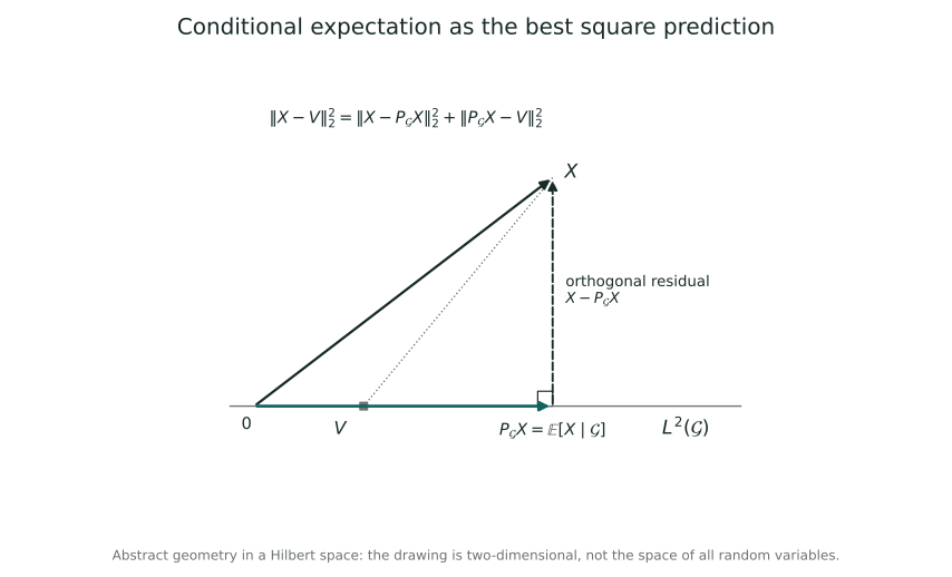
\mathcal H=L^2(\mathcal G)\subseteq L^2(\mathcal F).If Y\in\mathcal H is the conditional expectation, every bounded \mathcal G-measurable H satisfies
\langle X-Y,H\rangle=0.Truncate an arbitrary H\in\mathcal H, then use Cauchy–Schwarz to control the truncation error. The equality extends to every H\in\mathcal H.
The conditional-average requirement has become this: the error must be perpendicular to every available information direction.
If the error systematically points along some observable direction, we can adjust the price along that direction and reduce squared loss. A prediction that fully uses the information should leave no bias that the same information can correct.
This interpretation is attractive. Yet simply saying “take an orthogonal projection” would hide existence inside a name, much as saying “apply the extension theorem” could in the preceding chapter.
Two things must be checked: whether infinitely refined approximate predictions can escape the space, and whether increasingly good predictions actually have a best limit.
9.6 Can Predictions Become Arbitrarily Close and Yet Cease to Be Predictions at Their Limit?
Consider the first question.
Let X_n be Cauchy in L^2. Extract a subsequence such that
\|X_{n_{k+1}}-X_{n_k}\|_2\le2^{-k}.Then
\sum_k\mathbb E|X_{n_{k+1}}-X_{n_k}|
\le\sum_k2^{-k}<\infty.
Tonelli says the sum of absolute increments is finite almost everywhere. This subsequence therefore converges pointwise to a finite random variable X. Set it to 0 on the measurable null set of nonconvergence to obtain a measurable representative.
Furthermore, the finite triangle inequality and Fatou's lemma give
\|X-X_{n_k}\|_2
\le\sum_{j\ge k}2^{-j}\longrightarrow0.
Specifically, first bound the L^2 norm of a finite sum of increments, then let its upper endpoint increase; Fatou preserves the bound at the limit. This also ensures X\in L^2. The original Cauchy property then brings the whole sequence X_n to X in L^2.
This proves completeness of L^2.
The mechanism recalls Chapter 7: select a timeline with summable errors, obtain an almost sure limit, then carry norm control back to the whole sequence.
If every X_n is \mathcal G-measurable, the pointwise convergence event just used also belongs to \mathcal G. Defining the limit to be 0 on its complement still gives a \mathcal G-measurable representative.
Thus \mathcal H is itself complete and is a closed subspace of L^2(\mathcal F). Predictions based entirely on available information cannot approach a limit that requires extra information to express.
Closedness here does not assert a unique pointwise limit for every original representative. It asserts that, after identification up to almost sure equality, the norm limit still has a legitimate observable representative.
We can finally seek the best prediction without fearing that approximation will deprive it of a home.
9.7 How Is the Best Squared-Error Prediction Actually Constructed?
Set
d=\inf_{Z\in\mathcal H}\|X-Z\|_2.Since 0\in\mathcal H, the infimum is finite. Choose Y_n\in\mathcal H with \|X-Y_n\|_2\to d.
Could these predictions wander in different directions, each nearly attaining the minimum error without approaching one another?
The parallelogram identity prevents it:
\|Y_n-Y_m\|_2^2
=2\|X-Y_n\|_2^2+2\|X-Y_m\|_2^2
-4\left\|X-\frac{Y_n+Y_m}{2}\right\|_2^2.
Their midpoint is in \mathcal H, so the final squared norm is at least d^2. The right side therefore tends to 0. Nearly optimal predictions must be near one another; otherwise their midpoint would improve on the infimum.
Completeness and closedness make Y_n converge in L^2 to Y\in\mathcal H, with \|X-Y\|_2=d.
For any H\in\mathcal H, the point Y+tH is also in \mathcal H, so the real quadratic
\|X-Y-tH\|_2^2
=\|X-Y\|_2^2-2t\langle X-Y,H\rangle+t^2\|H\|_2^2
is minimized at t=0. Consequently,
\langle X-Y,H\rangle=0.Taking H=\mathbf1_A gives the integral equality on every A\in\mathcal G. Since Y\in L^2\subseteq L^1, it is precisely the conditional expectation we sought.
Projection is also unique: the difference of two such points belongs to \mathcal H and is perpendicular to \mathcal H, so its squared norm must vanish.
Existence in the square-integrable case is now more than a borrowed promise. Error minimization produced a Cauchy sequence; completeness retained its limit; and minimal error yielded the fair integral equalities.
Blockwise averages in finite partitions and orthogonal projection in an infinite-dimensional space are performing the same operation.
9.8 Does a Fair Average Still Exist When the Payoff Has No Finite Variance?
The second moment supplied geometry, but should not be an admission requirement for averaging.
Chapter 6 already allowed X to have only a finite first absolute moment. Requiring a finite variance merely to give information would exclude many payoffs we can already integrate.
First extract a property of the projected objects that does not involve squares.
If square-integrable V\ge0, its conditional expectation W is nonnegative too. Otherwise A=\{W<0\}\in\mathcal G would have \int_AW\,dP<0, contradicting \int_AV\,dP\ge0. The definition and uniqueness also give linearity, so projection preserves order.
Now let X\ge0, \mathbb E X<\infty, and take
X_n=X\wedge n,\qquad Y_n=\mathbb E[X_n\mid\mathcal G].Each X_n is bounded, so existence follows from the square-integrable case. Order preservation makes Y_n nonnegative and increasing; after removing one common \mathcal G-measurable null set, these inequalities hold for all integer n simultaneously.
Take the increasing limit Y. Monotone convergence gives
\mathbb E Y=\lim_n\mathbb E Y_n
=\lim_n\mathbb E X_n=\mathbb E X<\infty.
Thus Y is finite almost surely. Setting it to 0 on the possible null set of infinite values yields a \mathcal G-measurable integrable representative. For every A\in\mathcal G, monotone convergence again gives
\int_A Y\,dP
=\lim_n\int_A Y_n\,dP
=\lim_n\int_A X_n\,dP
=\int_A X\,dP.
For general real X\in L^1, decompose it as X^+-X^-, construct the two answers, and subtract. Uniqueness did not use second moments, so different constructions still agree almost surely.
We have obtained the full existence and uniqueness statement: on any probability space, for any sub-\sigma-algebra and any real integrable random variable, conditional expectation exists and is unique up to almost sure equality.
Neither the original space nor \mathcal G need be complete or countably generated. No regular conditional distribution was assumed, and no later martingale convergence theorem was borrowed.
Using the bounded \mathcal G-measurable weight \operatorname{sgn}(Y), we also obtain
\mathbb E|Y|
=\mathbb E[X\operatorname{sgn}(Y)]
\le\mathbb E|X|.
Together with linearity, this gives
\|\mathbb E[X\mid\mathcal G]-\mathbb E[Z\mid\mathcal G]\|_1
\le\|X-Z\|_1.
Squared-error geometry brought the object into being; truncation carried it into the whole integrable world. What remains is an operator that never enlarges mean absolute error.
9.8.1 If even the first average is infinite, can information still redistribute it?
Chapter 6 left us a game not covered by the preceding result: its return is nonnegative, every actual payment is finite, but its theoretical expectation is infinite.
We should not declare all conditioning meaningless merely because X\notin L^1. Nonnegative integration in Chapter 6 already allowed +\infty. What must be avoided is an undefined subtraction of positive and negative infinities.
Allow, therefore, a measurable X:\Omega\to[0,\infty], without requiring \mathbb E X<\infty. We truncate as before:
X_n=X\wedge n,\qquad Y_n=\mathbb E[X_n\mid\mathcal G].Each truncation is bounded, so the previous construction applies. Choose versions for which 0\le Y_n\uparrow outside one common \mathcal G-measurable null set, and set every Y_n to zero on that set. We can then define everywhere
Y=\lim_{n\to\infty}Y_n\in[0,\infty].This limit is \mathcal G-measurable. For every A\in\mathcal G, two applications of monotone convergence give
\int_A Y\,dP
=\lim_n\int_A Y_n\,dP
=\lim_n\int_A(X\wedge n)\,dP
=\int_A X\,dP.
Both sides of these equalities may be +\infty. This is the extended conditional expectation of a nonnegative random variable. When \mathbb E X<\infty, it agrees with the integrable conditional expectation; when expectation is infinite, Y need not be almost surely finite.
Uniqueness still holds, but we cannot immediately subtract two versions that may be infinite. Suppose Y,Z\ge0 both satisfy the definition, and take
A_m=\{Y<Z,\ Y\le m\}\in\mathcal G.Since \int_{A_m}Y\,dP\le m, the common event-integral condition makes \int_{A_m}Z\,dP finite as well. Only now do we subtract to obtain \int_{A_m}(Z-Y)\,dP=0. The difference is strictly positive on A_m, so P(A_m)=0. Taking the countable union over m, and interchanging Y,Z, proves almost-sure uniqueness, including infinite values. Thus any other nonnegative, bounded, increasing approximation to X gives the same answer.
Return to the particular payoff in Chapter 6:
P(X=2^k)=2^{-k},\quad k\ge1,
\qquad P(X<\infty)=1,\quad \mathbb E X=\infty.
If nothing is known, \mathcal G=\{\varnothing,\Omega\}, the conditional average must be constant. Its integral over \Omega forces
\mathbb E[X\mid\{\varnothing,\Omega\}]=+\infty
\quad\text{a.s.}
If the payoff itself has been observed, then
\mathbb E[X\mid\sigma(X)]=X<\infty
\quad\text{a.s.}
The same game has an infinite nonnegative average before its outcome is known, but only its finite payment remains once that outcome is observed. Information has not made an erroneous calculation with infinity. The infinite average came from many rare large payments; observing the actual outcome stops mixing those unresolved possibilities together.
An infinite expectation still does not automatically become a sensible real-world admission price: Chapter 6's distinctions concerning risk, wealth and pricing assumptions remain. Nor can this section turn a payoff with both positive and negative parts of infinite expectation into a conditional expectation by disguising \infty-\infty.
The construction also yields conditional monotone convergence without an integrable limit. If 0\le V_n\uparrow V, the increasing limit of the conditional averages preserves the integral of V on every A\in\mathcal G; the uniqueness just proved therefore gives
\mathbb E[V_n\mid\mathcal G]\uparrow\mathbb E[V\mid\mathcal G]
\quad\text{a.s.}
Section 9.13 will study limits under integrable control. For now, we retain this point: nonnegativity alone allows an average to reach infinity without destroying its meaning.
9.9 Why Can What We Already Know Be Taken Outside a Conditional Average?
Conditional expectation exists, so we no longer need to guess its formulas. Each property can be returned to its two requirements: observability and preservation of event integrals.
We first return to real integrable payoffs X, adding a second-moment assumption explicitly when squared loss is needed. Nonnegative extended objects remain available, but they cannot participate in signed subtraction without further checks.
If X is already \mathcal G-measurable, it is itself an admissible representative, so
\mathbb E[X\mid\mathcal G]=X\quad\text{almost surely}.Taking A=\Omega gives the total-expectation formula
\mathbb E\,\mathbb E[X\mid\mathcal G]=\mathbb E X.If X is independent of \mathcal G, every A\in\mathcal G satisfies
\mathbb E[X\mathbf1_A]=\mathbb E X\,P(A).Verify this first for nonnegative simple functions of X, then extend using truncation and limits of integrals. Thus
\mathbb E[X\mid\mathcal G]=\mathbb E X.An observation providing no related information cannot change the average. The converse generally fails, as we will see.
If H is bounded and \mathcal G-measurable, then
\mathbb E[HX\mid\mathcal G]
=H\,\mathbb E[X\mid\mathcal G].
The proof explains the formula. The right side is integrable and observable; for A\in\mathcal G, use the bounded weight H\mathbf1_A in the defining identity. The integrals agree immediately. A quantity already seen need not be averaged again over situations not yet seen.
This property also applies to unbounded H, but integrability must be checked. If H is real and \mathcal G-measurable, and HX\in L^1, order preservation gives
|\mathbb E[X\mid\mathcal G]|
\le\mathbb E[|X|\mid\mathcal G].
Truncate |H|, use the bounded-weight identity, then pass monotonically to the limit:
\mathbb E\!\left[|H|\,\mathbb E[|X|\mid\mathcal G]\right]
=\mathbb E|HX|<\infty.
The product on the right of the desired formula is therefore integrable too. Apply the existing identity to truncated H, then pass to the limit using L^1 contraction on one side and dominated convergence on the other. This proves the unbounded pull-out property.
The slogan that a known quantity is a constant has not been extended without limits. What permits it to be taken outside is the combination of measurability and integrability.
9.10 Why Does Seeing More and Then Forgetting Part Return the Same Average?
Imagine two observers at the game. One sees both completed games; the other sees only the first.
The first can know the final payoff. The second knows only its average in the situation visible to them. Averaging the first observer's answer using the second observer's information should agree with the second directly averaging the payoff.
The mathematical condition is that the information really is nested:
\mathcal H\subseteq\mathcal G\subseteq\mathcal F.Set Y=\mathbb E[X\mid\mathcal G], then Z=\mathbb E[Y\mid\mathcal H]. Every A\in\mathcal H also belongs to \mathcal G, so
\int_A Z\,dP=\int_A Y\,dP=\int_A X\,dP.Since Z is \mathcal H-measurable, uniqueness gives
\mathbb E[\mathbb E[X\mid\mathcal G]\mid\mathcal H]
=\mathbb E[X\mid\mathcal H].
This is the tower property. Conversely, a variable already averaged using less information can itself be read using more information, so
\mathbb E[\mathbb E[X\mid\mathcal H]\mid\mathcal G]
=\mathbb E[X\mid\mathcal H].
Inclusion does different work in these two equalities: in the first, every test event can pass through both integrals; in the second, the inner answer is already observable.
Without nesting, conditional expectations cannot be interchanged arbitrarily.
Take three equally likely sample points and X=(0,0,3). Let \mathcal G distinguish the third point from the first two, while \mathcal H distinguishes the first from the last two. Blockwise calculation gives
\mathbb E[X\mid\mathcal G]=(0,0,3),
\qquad
\mathbb E[X\mid\mathcal H]=(0,3/2,3/2).
Averaging once more,
\begin{aligned}
\mathbb E[\mathbb E[X\mid\mathcal G]\mid\mathcal H]
&=(0,3/2,3/2),\\
\mathbb E[\mathbb E[X\mid\mathcal H]\mid\mathcal G]
&=(3/4,3/4,3/2).
\end{aligned}
The answers differ.
Forgetting one detail and redistributing averages according to another classification can depend on the order. The tower property describes nested information, not two arbitrary averaging buttons that always commute.
9.11 Why Does Convexity Leave a Direction When Averaging Meets Nonlinearity?
Chapters 6 and 7 warned us that nonlinear operations do not generally pass through averages. Giving information does not change that.
For a convex function \varphi, however, there is a definite direction:
\varphi(\mathbb E[X\mid\mathcal G])
\le\mathbb E[\varphi(X)\mid\mathcal G]
\quad\text{almost surely}.
Here assume that \varphi:\mathbb R\to\mathbb R is finite and convex, X\in L^1, and \varphi(X)\in L^1. This specifies the integrals and avoids subtracting undefined infinities.
Why can a statement about an entire curve emerge from a conditional average?
A convex curve can be recovered from supporting lines below it. More precisely, choose a sequence of affine functions
\ell_j(x)=a_jx+b_j,\qquad
\ell_j\le\varphi,\qquad
\varphi(x)=\sup_{j\ge1}\ell_j(x).
It suffices to choose supporting slopes at rational points. A finite convex function is continuous inside every bounded interval; supporting slopes at nearby rational points are bounded between secant slopes on a slightly larger interval. Letting rational points approach x, the corresponding lines evaluated at x approach \varphi(x). A potentially uncountable family of supports has thus been reduced to a sequence.
For each line, order preservation and linearity give
a_j\mathbb E[X\mid\mathcal G]+b_j
\le\mathbb E[\varphi(X)\mid\mathcal G].
Countably many almost sure inequalities hold together on one full-probability set. Taking the supremum proves conditional Jensen.
It also proves integrability on the left: any one integrable affine function bounds it below, while the integrable variable on the right bounds it above. Both positive and negative parts are therefore integrable.
Countability again performs an unobtrusive but essential job. We cannot choose separate null sets for uncountably many lines and combine them without checking what remains.
Taking \varphi(x)=|x|^p, for 1\le p<\infty and X\in L^p, gives
|\mathbb E[X\mid\mathcal G]|^p
\le\mathbb E[|X|^p\mid\mathcal G],
\qquad
\|\mathbb E[X\mid\mathcal G]\|_p\le\|X\|_p.
For p=\infty, use -M\le X\le M and order preservation, then let M approach the essential bound.
This average respects all these error scales. It is not, however, optimal for every L^p loss: orthogonality has a special relationship with squared loss, whereas absolute loss is generally minimized by a conditional median. The squared-error conclusion cannot simply be generalized unchanged.
9.12 How Does the Remaining Randomness Separate from What Has Been Explained?
Return to X\in L^2 and write Y=\mathbb E[X\mid\mathcal G]. For every Z\in L^2(\mathcal G),
X-Z=(X-Y)+(Y-Z).The first term is orthogonal to all square-integrable \mathcal G-measurable variables; the second is one such variable. Expanding the square eliminates the cross term:
\mathbb E(X-Z)^2
=\mathbb E(X-Y)^2+\mathbb E(Y-Z)^2.
Thus Y has the smallest mean squared error among square-integrable predictions using this information. Another prediction attains the same minimum only when Z=Y almost surely.
This identity says more than “conditional expectation is optimal.” The extra loss from any other observable prediction is exactly its squared distance from the conditional average.
Write the variation not explained by the information as
\operatorname{Var}(X\mid\mathcal G)
=\mathbb E[(X-Y)^2\mid\mathcal G].
It is a nonnegative integrable random variable. Using L^2 contraction and the unbounded pull-out property established in Section 9.9, expand it to obtain
\operatorname{Var}(X\mid\mathcal G)
=\mathbb E[X^2\mid\mathcal G]-Y^2.
Here XY is integrable by Cauchy–Schwarz, and Y^2 is integrable by L^2 contraction. Taking Y outside therefore stays within the domain of integration.
Taking total expectations and adding and subtracting \mathbb E X gives
\operatorname{Var}(X)
=\mathbb E[\operatorname{Var}(X\mid\mathcal G)]
+\operatorname{Var}(\mathbb E[X\mid\mathcal G]).
Total variation splits into two parts: variation still present inside each known situation, and variation between the average values of different known situations.
Randomness has not merely become smaller. We have identified which differences the information can explain.
If \mathcal H\subseteq\mathcal G, the best prediction using \mathcal H also belongs to L^2(\mathcal G). More information cannot increase the minimum mean squared error:
\mathbb E\!\left(X-\mathbb E[X\mid\mathcal G]\right)^2
\le
\mathbb E\!\left(X-\mathbb E[X\mid\mathcal H]\right)^2.
This compares average losses. It does not assert that the two conditional variances are ordered at every sample point. Different information divides the world into different situations, and such a pointwise comparison has no general guarantee.
9.12.1 What Is the Difference between Knowing a Quantity and Being Allowed Only a Straight-Line Prediction?
Again let U be uniform on [-1,1], with payoff X=U^2.
Observing U completely gives
\mathbb E[X\mid\sigma(U)]=U^2.If we permit only predictions a+bU, the best answer is instead the constant 1/3. Symmetry gives \mathbb E U=\mathbb E U^3=0, while \mathbb E U^2=1/3. Expanding \mathbb E(U^2-a-bU)^2 shows its minimum at a=1/3,b=0.
These projections use different subspaces. Conditional expectation permits every square-integrable observable function; linear regression allows only linear combinations. Without additional structure, linear prediction cannot be identified with conditional expectation.
Conversely, if the payoff is U and we observe only U^2,
\mathbb E[U\mid\sigma(U^2)]=0.For every bounded Borel h, the function u\,h(u^2) is odd and integrates to 0 on the symmetric interval. This is exactly the bounded-test condition of the definition.
An unchanged average does not mean no information was gained. The event \{|U|\le1/2\}, of probability 1/2, is fully determined by U^2. If U and U^2 were independent, this event, belonging to both information systems, would intersect itself with probability 1/4; the actual probability is 1/2.
An unchanged conditional mean of one payoff says only that the observation has not changed its average. Independence requires separation of the probabilities of all measurable events, a far stronger condition.
9.13 What Happens to Chapter 7's Spike after Information Is Given?
We know how to take one conditional average. If the payoff changes through approximation, will its conditional average stabilize too?
For L^1 convergence, contraction answers immediately:
X_n\longrightarrow X\text{ in }L^1
\quad\Longrightarrow\quad
\mathbb E[X_n\mid\mathcal G]
\longrightarrow\mathbb E[X\mid\mathcal G]\text{ in }L^1.
The same argument works for L^p convergence with finite p\ge1. The information \mathcal G is fixed here; increasing information systems pose a different limit question.
Almost sure convergence alone can fail to give the answer.
On (0,1) with Lebesgue probability, let
X_n=n\mathbf1_{(0,1/n)}.This tends to 0 almost everywhere, but \mathbb E X_n=1. If \mathcal G=\{\varnothing,\Omega\} tells us nothing,
\mathbb E[X_n\mid\mathcal G]=1at every stage.
Chapter 6's spike has not disappeared because the word “conditional” was added. Without adequate tail control, convergence of individual records can still fail to carry the average. Chapter 7's uniform integrability reconnects precisely here: convergence in probability plus UI gives L^1 convergence, which carries conditional averages to their limit in L^1.
Dominated convergence gives a stronger conclusion, along individual records.
First consider conditional monotone convergence. If 0\le V_n\uparrow V with V\in L^1, order preservation makes \mathbb E[V_n\mid\mathcal G] increasing. Its limit has total expectation at most \mathbb E V, and monotone convergence makes its integral on every A\in\mathcal G equal to \int_AV\,dP. Uniqueness gives
\mathbb E[V_n\mid\mathcal G]\uparrow\mathbb E[V\mid\mathcal G]
\quad\text{almost surely}.
If X_n\to X almost surely and |X_n|\le Z\in L^1, then |X|\le Z on a common full-probability set. Define
R_n=\sup_{k\ge n}|X_k-X|.Then 0\le R_n\le2Z and R_n\downarrow0 almost surely. Apply the monotone conclusion to R_1-R_n\uparrow R_1 to obtain
\mathbb E[R_n\mid\mathcal G]\downarrow0
\quad\text{almost surely}.
Moreover,
\left|\mathbb E[X_n\mid\mathcal G]-\mathbb E[X\mid\mathcal G]\right|
\le\mathbb E[R_n\mid\mathcal G].
This proves conditional dominated convergence: the conditional expectations converge almost surely. Ordinary dominated convergence and L^1 contraction also give their L^1 convergence.
Why introduce the supremum of the entire tail? Vanishing average error at each stage directly gives only L^1 control. A tail envelope bounds all future errors together, allowing eventual quietness along individual records.
The four kinds of convergence remain different inside conditional averaging. Conditional expectation does not erase these distinctions; it reveals which limits really preserve averages.
9.14 How Does Chapter 2's Coin Enter One Infinite Probability World?
Return now to the coin whose probability of heads is unknown.
Chapter 2 computed posteriors from finite records. Chapter 8 allows the unknown parameter and infinite record to coexist, rather than requiring a temporary model for each calculation.
Let \Theta\in[0,1] be the unknown heads probability, initially with a uniform prior. For each finite record x_1,\ldots,x_n\in\{0,1\}, prescribe the joint probability
P(\Theta\in d\theta,\ X_1=x_1,\ldots,X_n=x_n)
=\theta^{s}(1-\theta)^{n-s}\,d\theta,
\qquad s=\sum_{j=1}^n x_j.
At endpoints the powers are interpreted through the product of Bernoulli probabilities. Summing over all records gives total mass 1; removing the last entry contributes the factor \theta+(1-\theta)=1. These finite rules are therefore consistent.
Combine the parameter coordinate and successive coin coordinates in a countable product. Chapter 8's standard Borel extension supplies a common probability space. We did not first assume the existence of general conditional-distribution kernels: we wrote finite joint rules and let extension perform the existence work.
Write
\mathcal F_n=\sigma(X_1,\ldots,X_n),
\qquad S_n=X_1+\cdots+X_n.
Every finite record has positive probability. The partition formula of Section 9.2 gives
\mathbb E[\Theta\mid\mathcal F_n]
=
\frac{\int_0^1\theta^{S_n+1}(1-\theta)^{n-S_n}\,d\theta}
{\int_0^1\theta^{S_n}(1-\theta)^{n-S_n}\,d\theta}.
The ratio can be calculated completely. For nonnegative integers a,b, set
I_{a,b}=\int_0^1\theta^a(1-\theta)^b\,d\theta.For b\ge1, integration by parts, with zero boundary terms, gives
I_{a,b}=\frac{b}{a+1}I_{a+1,b-1}.Starting from I_{a,0}=1/(a+1) and substituting repeatedly yields
I_{a,b}=\frac{a!\,b!}{(a+b+1)!}.Hence
M_n:=\mathbb E[\Theta\mid\mathcal F_n]
=\frac{S_n+1}{n+2}.
The order of a finite record may change, but its conditional average stays the same when the number of heads does. Remembering only the count is a fact calculated from this joint model and these integrals, not an unproved appeal to general statistical sufficiency.
Use the same joint rule directly for the next coin:
P(X_{n+1}=1\mid\mathcal F_n)=\frac{S_n+1}{n+2}=M_n.The numerator gains one factor of \theta compared with the probability of the current record, giving exactly the same ratio of integrals. In this model, the conditional mean of the unknown parameter unifies with the predictive probability of the next success.
This does not require every unknown real-world coin to have a uniform prior. It says that once a joint probability has been specified, inference, prediction, and averaging given information must agree within the same accounts.
9.15 How Can a Judgment Keep Changing and Still Be a Fair Game?
Continue watching M_n.
A first head raises it from 1/2 to 2/3; a tail lowers it to 1/3. Later records change it again. We do not have a pointwise monotone sequence of judgments.
Ideas about fair gambling are much older than modern martingale theory; the two should not simply be identified. Ville's 1939 book examined random collectives through gambling strategies. Doob later recalled being stimulated, while reviewing it, by its maximum inequality and argument for the Bernoulli strong law. Ville's original work · Doob's interview.
In his 1935 work on random series, Lévy also studied conditional probabilities based on successive observations and their limits. In modern language this was an early route toward martingale limit theory, not a claim that his paper already used our complete definitions. Lévy's original paper. Doob organized fairness, increasing information and random observation times into a systematic theory, developed extensively in his 1953 Stochastic Processes. The equality below therefore connects an old problem to a structure clarified much later; its entire content cannot be attributed to some ancient game.
The tower property nevertheless guarantees
\mathbb E[M_{n+1}\mid\mathcal F_n]
=\mathbb E[\mathbb E[\Theta\mid\mathcal F_{n+1}]\mid\mathcal F_n]
=\mathbb E[\Theta\mid\mathcal F_n]
=M_n.
Given present information, the next update has no systematic upward or downward bias.
More generally, let information increase:
\mathcal F_0\subseteq\mathcal F_1\subseteq\cdots.Such an information flow is a filtration. For any integrable final payoff X, let
M_n=\mathbb E[X\mid\mathcal F_n].Each M_n is integrable and \mathcal F_n-measurable, and satisfies the same fairness equality. This is the basic structure of a martingale: observable in its own information flow, with next-step conditional average equal to the present value.
We encounter it here without importing every martingale theorem at once. What has truly appeared is a new question.
As information grows, will these recalculated prices stabilize? If
\mathcal F_\infty=\sigma\left(\bigcup_n\mathcal F_n\right),do we have
M_n\longrightarrow\mathbb E[X\mid\mathcal F_\infty]?In which sense of convergence? Is integrability enough? What connects increasing information with Chapter 7's control of tails?
The tower identity itself proves none of this. A process fair at every step still needs a limit theory, and eventually knowing all information requires specifying what that information contains.
For the coin model we can further ask whether the entire record almost surely identifies \Theta. This links conditioning to laws of large numbers for independent sequences. We have seen where the theories meet; reaching an interface is not the same as completing every road.
The fair game of Chapter 1 is no longer confined to a stake. A judgment continually absorbing new observations can itself be a fair process.
9.16 Once Conditional Means Exist, Do We Already Have a Probability World at Every Observation?
For A\in\mathcal F, define
P(A\mid\mathcal G)=\mathbb E[\mathbf1_A\mid\mathcal G].Order preservation places it between 0 and 1 almost surely. For disjoint events A_j, finite linearity and conditional monotone convergence give
P\left(\bigcup_{j\ge1}A_j\mid\mathcal G\right)
=\sum_{j\ge1}P(A_j\mid\mathcal G)
\quad\text{almost surely}.
Every prescribed countable relation holds after a null set is removed.
This does not automatically supply a map satisfying all probability axioms simultaneously at each sample point:
(\omega,A)\longmapsto K(\omega,A).Versions for different events may use different exceptional sets, as may different countable relations. We cannot combine the null sets of uncountably many requirements and declare that one common full-probability world remains.
If such a K exists, with A\mapsto K(\omega,A) a probability for every \omega, and \omega\mapsto K(\omega,A) a \mathcal G-measurable version of the conditional probability for every A, then we have the corresponding regular conditional probability kernel. Constructing conditional-distribution kernels for random elements in standard Borel spaces is a more structured existence result still to be established; it cannot be transferred without conditions to arbitrary original measurable spaces.
Even for a real observation Z, point values require care.
A real \sigma(Z)-measurable variable Y can indeed be written as a Borel function g of Z:
Y=g(Z).This measurable factorization has a direct proof. Approximate Y pointwise by \sigma(Z)-measurable simple functions. Every level set is Z^{-1}(B), so each simple function is a Borel simple function of Z. Take the limit of these Borel functions where it exists and is finite, and set it to 0 elsewhere. The resulting g is Borel, and the inverse-image representations ensure it yields Y pointwise on Z(\Omega).
Thus \mathbb E[X\mid\sigma(Z)] can be written g(Z), but g is determined only almost everywhere under the law of Z.
If Z has a continuous distribution, changing g(z_0) at a fixed point z_0 may give the same conditional-expectation version. Without a version convention or additional continuous structure, “given Z=z_0” cannot mean a uniquely determined pointwise answer.
For example, with X=U and Z=U, we can choose g(u)=u. Changing g at a fixed probability-zero point still leaves g(U) equal to U almost surely. A natural expression may be excellent without being the only mathematically permissible version.
The definition has not been lost. Clarifying the almost sure object is precisely what allows us to ask which pointwise structures should be retained and which can be proved to exist.
9.17 Why Does a New Density Appear inside Information?
For nonnegative integrable X, define a measure on \mathcal G by
\nu(A)=\int_A X\,dP,\qquad A\in\mathcal G.It is countably additive, and P(A)=0 implies \nu(A)=0. Hence
\nu\ll P|_{\mathcal G}.The defining property of Y says exactly that
\nu(A)=\int_A Y\,dP\quad(A\in\mathcal G).Thus Y is the density of this measure relative to the original probability restricted to known information.
Chapter 6 unified discrete weights and Lebesgue integration. Conditional averaging has now brought us to comparing measures: can one measure be expressed by weighting another?
Radon–Nikodym theory will answer that question systematically. We have proved existence of the particular density needed for conditional expectation, not yet the general density theorem for arbitrary absolutely continuous measures. We have not borrowed the general theorem to obtain conditional expectation and then used that same conditional expectation as a disguised proof of the general theorem.
For a real observation Z, we may also move the accounts to the observation space. Write its law as \mu_Z, and define
\nu_Z(B)=\mathbb E[X\mathbf1_{\{Z\in B\}}],
\qquad B\in\mathcal B(\mathbb R).
If Y=g(Z) is the conditional expectation, change of variables gives
\nu_Z(B)=\int_Bg(z)\,\mu_Z(dz).The natural order of the theory now appears: establish densities between measures, organize conditional events into a probability kernel, and finally let that kernel choose successive experiments.
Chapter 8 moved from finite windows to a common probability; Chapter 9 distinguished known from unknown inside that probability. Constructing kernels will join the two roads, making selection of the next step from the present state into an infinite experiment whose existence can actually be proved.
Chapter 9 Epilogue: Fairness Is Not Knowing the Future, but Making Full Use of What Is Known
Let us return one last time to the 64 coins on the table.
Conditional expectation does not let anyone predict the unfinished match. The final payoff remains random; the winner has not appeared.
We have gained a different ability: whenever a new situation becomes visible, recalculate a price using only that situation, preserving the same average as the actual payoff on every event that situation allows us to recognize.
Blockwise division in finite partitions once made this seem like a few lines of arithmetic. Continuous observations turned denominators into zero and forced the condition to move from points to event systems. Squared error turned fairness on events into orthogonality; completeness retained limits of improving predictions; truncation carried this average beyond the finite-variance boundary.
Fair pricing from Chapter 1, Bayesian updating from Chapter 2, integration from Chapter 6, and limit control from Chapter 7 have met in one object.
The same expectation can be recalculated at different information levels. More observation does not make every judgment move in one direction. It makes more distinctions recognizable, so known details need no longer remain mixed with unknown variation.
If we want not merely an average but the conditional law of every future outcome, these separately existing answers must become a compatible probability. If the next experiment depends on the present state, that probability must also vary measurably with the state.
We stand at a familiar threshold again: does having an answer to each question separately ensure that all answers form one world together?
The next chapter starts from relative densities between measures and moves toward conditional distributions and probability kernels. We will no longer just assemble windows into records; we will understand how the next step of a record is chosen when information changes.
The infinite world has a home. We are beginning to learn how to observe within it.
History and Further Reading
The division-of-stakes problem in Chapter 1 and the Bayesian coin in Chapter 2 supply this chapter's historical problems. Its four-record example, information language of \sigma-algebras, geometric construction, and posterior process are modern reconstructions, not abstract theories attributed to Pascal, Fermat, or Bayes in their own time.
Kolmogorov's 1933 book places a chapter on conditional probabilities and expectations after mathematical expectations. This verifiable table-of-contents fact establishes conditioning as an explicit theme of his foundations; it does not make our projection proof a reproduction of his book. Original book record and contents.
For modern definitions and theoretical connections, compare MIT 18.175, Scott Sheffield, conditional expectation lecture notes. Our proofs develop from the integration, convergence, and infinite experiments established earlier; the book's own problems determine the arrangement of finite partitions, the L2 construction, L1 truncation, and limits of information.
The reference for theoretical breadth remains Kallenberg, Foundations of Modern Probability, third edition. Official bibliography and contents. We use it to check the range connecting conditioning, measure decomposition, kernels, and later processes, without transferring its prose or chapter progression.
The martingale history in the text is checked against Ville's original work, Lévy's 1935 paper and Doob's own interview. Early conditional-probability limits are distinguished from the systematic modern language of filtrations, stopping times and martingales. The payoff, projection and truncation arguments here remain modern mathematical reconstructions.