Haobai Wang · Public reading edition · ch02-en-877bf501293c
This content fingerprint identifies the text, not academic final approval or an independent proof of authorship.
SHA-256: 877bf501293c0c9ac633c55b9b104a9e0e483bd705a21b3f5421b01620fde578
The Mathematics of Chance
Volume I · Can Chance Be Calculated?
Chapter 2: From Chance to Knowledge—How Do We Discover Unknown Probabilities?
From Jacob Bernoulli's law of large numbers to Thomas Bayes's inverse inference.
In Chapter 1, we discovered something surprising.
An unfinished game of chance forced us to consider fairness, chance, and why a future that has not yet occurred can become an object of mathematical study.
Yet the theory we developed always depended on a special condition:
We knew the chances of the different outcomes in advance.
For a fair die, we assumed that all six faces were equally likely. For a fair coin, we assumed that heads and tails had the same probability.
What happens if we no longer know those probabilities?
This time, we cannot move directly from a mathematical model to its outcomes.
We must start from outcomes already observed and work backward to understand the unknown law that generated them.
This will bring a fundamental change to probability theory.
2.1 An Unfair Coin
Imagine that someone hands us a coin.
We do not know whether it is fair or whether someone has altered it.
We know only that each toss produces heads or tails.
Let the probability of heads be
p.Unlike in Chapter 1, however, we do not know the value of p.
All we can be sure of is
0\le p\le1.The question now is:
Can observing the coin's actual behavior tell us the value of p?
Suppose we toss it ten times and obtain seven heads and three tails.
A very natural answer is:
p\approx\frac7{10}=0.7.But what mathematical basis does this answer have?
If the true value is p=1/2, seven heads in ten tosses is entirely possible.
If the true value is p=0.8, seven heads is also entirely possible.
Even when p=0.3, seven heads is still an event with nonzero probability.
Thus:
\text{observing seven heads}
\not\implies p=0.7.
At most, we can say that some values of p seem to fit the observation better than others.
But what does “fit better” mean?
Before answering, we need to recognize a more fundamental distinction.
2.2 Two Very Different Kinds of Uncertainty
We have encountered two questions pointing in opposite directions.
First question: given the probability, predict the outcomes.
If we know that the probability of heads is p, we want to calculate the probability of seven heads in the next ten tosses.
This is a forward probability problem.
Second question: given the outcomes, infer the probability.
If we have observed seven heads in ten tosses, we want to infer the unknown p.
This is a problem of inverse inference.
In modern notation, let
X_i=
\begin{cases}
1,&\text{trial }i\text{ is heads},\\
0,&\text{trial }i\text{ is tails}.
\end{cases}
For a given p, assume
X_1,\ldots,X_n
\overset{\mathrm{i.i.d.}}{\sim}\operatorname{Bernoulli}(p).
Define
S_n=\sum_{i=1}^n X_i.The forward problem studies
P_p(S_n=k).The inverse problem asks:
after observing S_n=k, what can we conclude about p?
Although they seem merely to exchange the known and the unknown, the two questions differ substantially in mathematical terms.
In the first, the probability model has already been specified.
In the second, we are trying to understand the probability model itself.
Forward problem
p\text{ known}P_p(S_n=k)From law to observation
Inverse problem
S_n=k\text{ known}p\text{ unknown}From observation to law
Historically, the move from the mathematics of gambling to inference about the real world was a major turning point in the development of probability.
In dice games, rules and symmetry can give us probabilities.
For human lifespans, disease rates, natural phenomena, or social events, however, we often have no reason to assume equal likelihood in advance.
All we have is what happened in the past.
If probability theory could handle only problems with known probabilities, it could never become a mathematics of the empirical world.
Jacob Bernoulli recognized precisely this important direction.
2.3 Jacob Bernoulli: Can Experience Reveal Probability?
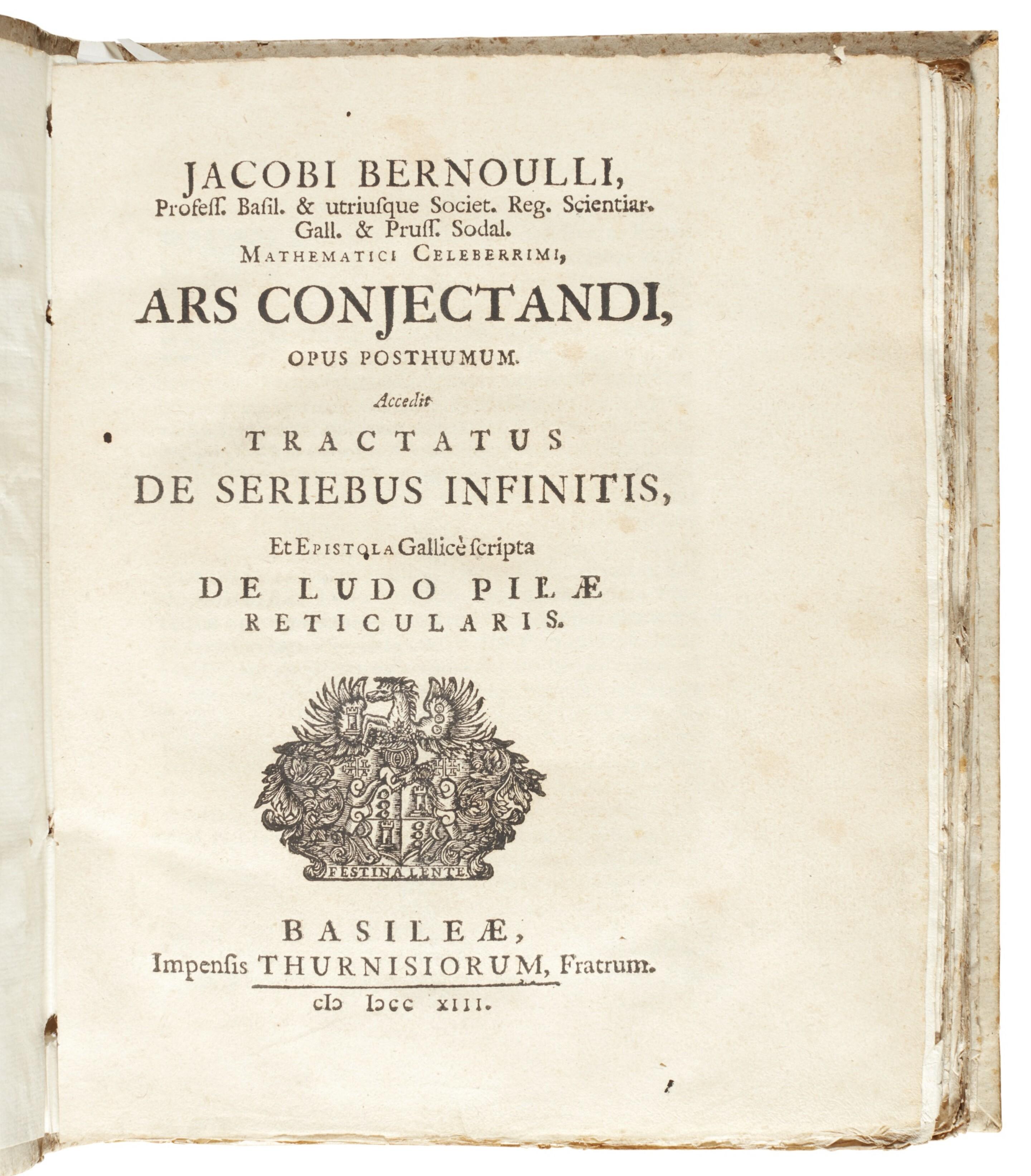
Jacob Bernoulli(1655—1705)
A Swiss mathematician and an important member of the Bernoulli family, he spent many years studying how to extend the mathematics of games of chance to uncertain problems in everyday life.
His book Ars Conjectandi (The Art of Conjecturing) was published posthumously in 1713.
The book matters for more than its inclusion of what later became known as the law of large numbers.
Still more significant is the question Bernoulli was trying to answer.
In his day, mathematicians could calculate chances in idealized games because the rules were usually known.
The real world, however, does not tell us its probabilities in advance.
For example:
How likely is a particular disease to be fatal?
What proportion of a population has a certain characteristic?
How frequently will a natural phenomenon occur under specified conditions?
Can repeated observation gradually reveal these unknown proportions?
In Ars Conjectandi, Bernoulli sought to extend the mathematics of gambling to civil, moral, and economic matters. His law of large numbers provided a mathematical basis for inferring unknown chances from repeated observations. Historians Edith Dudley Sylla and Ian Hacking have both emphasized the significance of this move from gambling to empirical inference. 〔11, 12, 13〕
But an apparent paradox arises.
If we do not know p to begin with, how can we prove that observed frequencies will get closer and closer to p?
We seem to need to know the probability before we can justify discovering it through observation.
This was the central mathematical problem Bernoulli faced.
2.3.1 Begin with an Urn Whose Proportions Are Known
Consider an urn containing r red balls and s black balls.
Each time, draw a ball at random, record its color, put it back, and mix the contents again.
Assume that every ball has the same chance of being drawn.
The probability of drawing red is then
p=\frac{r}{r+s}.Make n independent repeated draws.
Define
X_i=\mathbf1_{\{\text{trial }i\text{ draws a red ball}\}}.The number of red balls drawn is
S_n=X_1+\cdots+X_n.so the empirical frequency is
\widehat p_n=\frac{S_n}{n}.We are not asking whether, for some particular finite n, it equals p exactly.
Even when p=1/2, ten red draws in a row are entirely possible.
The real question is:
for any given accuracy \varepsilon>0, as the number of trials increases, does
|\widehat p_n-p|<\varepsilonhold with increasingly high probability?
In modern mathematical language, we want to prove:
\boxed{
P_p\left(
\left|\frac{S_n}{n}-p\right|>\varepsilon
\right)\longrightarrow0.
}
This is the modern form of Bernoulli's law of large numbers.
More precisely, it expresses convergence in probability:
\boxed{
\widehat p_n\xrightarrow{P_p}p.
}
Bernoulli proved an early rigorous form of this idea. He studied not only the limit, but also how to make the probability of a deviation smaller than a prescribed number. His argument used the binomial distribution and combinatorics rather than the modern variance inequality we will use next. 〔14, 13〕
2.4 Why Can Random Error Disappear?
Let us leave history for a moment and prove this phenomenon anew using modern mathematics.
There is something here well worth considering.
Every toss is random.
Even after a million trials, the million-and-first outcome may still be heads or tails.
If randomness in individual outcomes does not disappear, why can their average become increasingly stable?
The answer lies in the different properties of expectation and variance.
Step One: From the Total Count to the Average
Since
X_i\sim\operatorname{Bernoulli}(p),we have
\mathbb E_p[X_i]
=
1\cdot p+0\cdot(1-p)
=p.
Therefore
\mathbb E_p[\widehat p_n]
=
\mathbb E_p\left[\frac1n\sum_{i=1}^nX_i\right]
=p.
The expectation of the empirical frequency always equals the true probability.
But this alone does not allow us to claim that the empirical frequency will be close to the true probability.
For when n=1,
\widehat p_1\in\{0,1\},its expectation is still p, yet its value may be far from p.
Expectation tells us a random quantity's average location, but cannot by itself tell us how strongly it fluctuates around that location.
We are therefore forced to study the fluctuations themselves.
Step Two: Measure Fluctuations with Variance
For a Bernoulli random variable,
X_i^2=X_i.Thus
\begin{aligned}
\operatorname{Var}_p(X_i)
&=\mathbb E_p[X_i^2]-(\mathbb E_p[X_i])^2\\
&=p-p^2\\
&=p(1-p).
\end{aligned}
Next consider the variance of the average.
In general,
\operatorname{Var}\left(\sum_{i=1}^nX_i\right)
=
\sum_{i=1}^n\operatorname{Var}(X_i)
+
2\sum_{i<j}\operatorname{Cov}(X_i,X_j).
Since we assumed independent draws,
\operatorname{Cov}(X_i,X_j)=0,\qquad i\ne j.Hence
\operatorname{Var}_p(S_n)=np(1-p).Therefore
\boxed{
\operatorname{Var}_p(\widehat p_n)
=
\frac{p(1-p)}n.
}
This is the heart of the proof.
If we consider only the number of successes S_n, its variance increases with n.
But the variance of the relative frequency of success S_n/n decreases at the rate 1/n.
Expressed as a standard deviation, the typical scale of these fluctuations is
\boxed{
\sqrt{\operatorname{Var}(\widehat p_n)}
=
\sqrt{\frac{p(1-p)}n}.
}Theoretical values,with p = 0.5;the vertical axis represents frequency rather than the total number of successes。
查看母稿数值表
| n | Standard deviation |
|---|---|
| 1 | 0.5 |
| 5 | 0.223607 |
| 10 | 0.158114 |
| 20 | 0.111803 |
| 50 | 0.070711 |
| 100 | 0.05 |
| 200 | 0.035355 |
| 500 | 0.022361 |
| 1000 | 0.015811 |
An important mathematical phenomenon appears here:
to halve the standard deviation, we generally need to quadruple the sample size.
This is because
\operatorname{SD}(\widehat p_n)\propto\frac1{\sqrt n}.This provides the simplest example of the \sqrt n scale that will appear so often in statistical inference.
Of course, we have studied only second moments so far; we have not proved a more detailed limiting distribution.
Step Three: From Mean Squared Error to a Probability Statement
We already know
\mathbb E_p[(\widehat p_n-p)^2]
=
\frac{p(1-p)}n.
But the law of large numbers requires control of
P_p(|\widehat p_n-p|\ge\varepsilon).How can we turn a statement about expectation into a statement about probability?
Notice that for every real number y,
\mathbf1_{\{|y|\ge\varepsilon\}}
\le\frac{y^2}{\varepsilon^2}.
Therefore
\begin{aligned}
P_p(|\widehat p_n-p|\ge\varepsilon)
&=\mathbb E_p\left[
\mathbf1_{\{|\widehat p_n-p|\ge\varepsilon\}}
\right]\\
&\le
\frac{\mathbb E_p[(\widehat p_n-p)^2]}
{\varepsilon^2}\\
&=\frac{p(1-p)}{n\varepsilon^2}.
\end{aligned}
Since
p(1-p)\le\frac14,we obtain
\boxed{
P_p(|\widehat p_n-p|\ge\varepsilon)
\le\frac1{4n\varepsilon^2}.
}
For each fixed \varepsilon>0, the right-hand side tends to zero.
Thus
\boxed{\widehat p_n\xrightarrow{P_p}p.}This completes the proof.
The proof is short, but it reveals a deep structure.
We have not made individual random events deterministic.
We have proved only that averaging sufficiently many independent random events constrains the fluctuations of their average more and more tightly.
Randomness has not disappeared; what disappears is the chance that the average deviates from its center.
2.4.1 Where Exactly Does Independence Enter?
Look at the proof again.
The expectation step,
\mathbb E\left[\frac1n\sum X_i\right]
=
\frac1n\sum\mathbb E[X_i]
does not require independence.
Independence is actually used in
\operatorname{Var}\left(\sum X_i\right)
=
\sum\operatorname{Var}(X_i).
If the random variables are correlated, their covariances may not be negligible.
For example, suppose
X_1=X_2=\cdots=Yand Y\sim\operatorname{Bernoulli}(p).
All trial outcomes are then identical.
Although each X_i still has marginal distribution Bernoulli(p),
\widehat p_n=Yfor every n.
Increasing the number of repetitions therefore produces no stabilization at all.
The law of large numbers thus depends on more than the surface fact that “we performed many trials.”
More fundamentally, the dependence among trials must be weak enough to control the average error.
Independence is a particularly effective sufficient condition, but it is not the only possible hypothesis for a law of large numbers.
We will return to this question repeatedly when studying ergodic theory, martingales, and dependent stochastic processes.
2.5 What Does the Law of Large Numbers Answer, and What Does It Leave Open?
We have now proved an important conclusion:
\widehat p_n\xrightarrow{P_p}p.At first sight, this seems to solve the problem of inferring an unknown probability.
If we observe enough trials, the empirical frequency will approach the true probability.
But a logical difficulty is hidden here.
The law of large numbers says:
Assuming the true probability is
p, the empirical frequency is likely to be close top.
What we want to conclude is:
I have observed an empirical frequency of
0.7, so the true probability should be close to0.7.
These statements look similar, but they are not the same logical proposition.
One predicts observations from a model.
The other infers a model from observations.
We cannot simply reverse the direction of a conditional probability statement without proof.
2.5.1 How Can the Law of Large Numbers Become an Actual Method of Inference?
Fortunately, its probability inequality provides a more rigorous approach.
We proved earlier that
P_p(|\widehat p_n-p|\ge\varepsilon)
\le\frac1{4n\varepsilon^2}.
Notice that the inequality holds for every p\in[0,1].
Even without knowing p, we can therefore prescribe an acceptable error probability \delta\in(0,1) in advance.
Set
\varepsilon_n=\sqrt{\frac1{4n\delta}}.Then
P_p\left(
|\widehat p_n-p|\le\varepsilon_n
\right)\ge1-\delta.
Now define a random interval determined by the observed data:
\boxed{
C_n=
\left[
\widehat p_n-\varepsilon_n,
\widehat p_n+\varepsilon_n
\right]\cap[0,1].
}
For every true parameter p, we then have
\boxed{
P_p(p\in C_n)\ge1-\delta.
}
This is a parameter-inference procedure with a rigorous coverage guarantee.
For example, suppose we make 100 independent tosses and observe 70 heads.
Take \delta=0.05.
Then
\varepsilon_{100}
=
\sqrt{\frac1{4(100)(0.05)}}
\approx0.224.
giving the interval
C_{100}\approx[0.476,0.924].This interval is indeed very wide.
Its advantage, however, is a coverage guarantee of at least 95%, obtained without any prior guess about the unknown p.
Modern statistics can improve this substantially through sharper inequalities or exact binomial methods. This construction is intended only to make the mathematical principle clear.
2.5.2 A Subtle Philosophical Question
Now suppose we have indeed observed 70 heads and calculated this fixed interval.
Can we say:
“The probability that the true parameter lies in this interval is at least 95%”?
That interpretation does not follow directly within the mathematical framework just used.
The reason is that p is treated as a fixed but unknown parameter.
Before the experiment, the interval C_n is random. It may or may not contain the true parameter.
Once we observe particular data, however, the interval is determined.
Coverage means: if we repeatedly use this construction in repeated experiments with the same true parameter, at least 95% of the intervals will contain it.
It does not directly assign a 95% conditional probability to the already fixed parameter.
Yet from the practical human position of facing an unknown, another question is almost inevitable:
since we do not know p, why can we not assign a probability to p itself?
For example:
P(0.6<p<0.8\mid\text{observed data})=?This requires a mathematical structure different from the fixed-parameter model above.
The “unknown probability” itself must become an object of probabilistic inference.
Historically, Thomas Bayes took a crucial step in this direction.
2.6 Thomas Bayes: Can Probability Itself Be Uncertain?
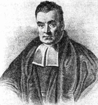
Thomas Bayes (c. 1701–1761)
An English minister and mathematician.
After his death, Richard Price edited his paper An Essay towards Solving a Problem in the Doctrine of Chances and submitted it to the Royal Society. It appeared in the 1763 volume of the Philosophical Transactions.
The paper's starting point is remarkably close to our question.
Suppose an event has occurred a certain number of times and failed to occur a certain number of times.
Knowing only these observations, can we calculate the chance that its probability of occurrence lies between two given values?
Bayes studied precisely this kind of interval probability inference for an unknown success probability. 〔15, 16, 17〕
A historical distinction is needed here.
The familiar Bayes formula,
P(H\mid D)
=
\frac{P(D\mid H)P(H)}{P(D)},
was not a conditional probability identity that first appeared in his paper wholly independently of earlier mathematical developments.
Bayes's important contribution was a concrete probabilistic analysis of the inverse problem of unknown chances.
Nor did he simply declare that “all unknown parameters should be uniformly distributed.” He constructed a physical model in which the random landing position of a ball generated an unknown probability, thereby giving his particular problem an initial probability structure. Historians have also discussed carefully the relationship between his original argument and later Bayesian thought. 〔18, 19, 20〕
We now reconstruct this idea in modern probability language.
2.6.1 A New Experiment: First Choose the Coin's Bias at Random
Imagine that we design a device.
First, choose a number uniformly at random from [0,1].
Call this number
\Theta.Thus
\Theta\sim\operatorname{Uniform}(0,1).Second, use the randomly chosen number to manufacture a coin whose probability of heads is exactly \Theta.
Third, toss this coin many times independently.
Notice that we do not manufacture a new coin for every toss.
Once chosen, \Theta becomes the fixed bias of this coin.
We therefore obtain the following hierarchical model:
\boxed{
\begin{aligned}
\Theta&\sim\operatorname{Uniform}(0,1),\\
X_i\mid\Theta=\theta
&\overset{\mathrm{i.i.d.}}{\sim}
\operatorname{Bernoulli}(\theta).
\end{aligned}
}
There is an important difference between this model and the preceding section's.
Previously, p was a fixed but unknown number.
Now, \Theta is an actual random variable.
We can therefore legitimately ask:
P(\Theta\in[a,b]).Before observing any data,
P(\Theta\in[a,b])=b-a,
\qquad 0\le a\le b\le1.
In modern terminology, this is called the prior distribution.
In our device, however, it does more than express subjective belief.
It has a clear physical interpretation: we actually generated an unknown parameter by a uniform random mechanism.
Assigning probabilities to unknown parameters therefore does not necessarily imply a subjective interpretation of probability; its meaning depends on how the model is constructed.
2.7 How Do Observations Change the Distribution of an Unknown Probability?
Now suppose we toss this coin ten times and observe seven heads.
Define
S_{10}=X_1+\cdots+X_{10}.We know
S_{10}=7.and want to calculate
P(\Theta\in[a,b]\mid S_{10}=7).First, given \Theta=\theta, the ten tosses are independent, so
P(S_{10}=7\mid\Theta=\theta)
=
\binom{10}{7}\theta^7(1-\theta)^3.
Now apply the idea of conditional probability.
If the prior density is \pi(\theta), then after observing data D, the posterior density must satisfy
\pi(\theta\mid D)
=
\frac{P(D\mid\theta)\pi(\theta)}
{\int_0^1P(D\mid u)\pi(u)\,du}.
In our uniform-prior model,
\pi(\theta)=1,\qquad 0<\theta<1.Hence
\pi(\theta\mid S_{10}=7)
=
\frac{\theta^7(1-\theta)^3}
{\int_0^1u^7(1-u)^3\,du}.
The denominator is a beta integral:
\int_0^1u^7(1-u)^3\,du
=
B(8,4)
=
\frac{7!\,3!}{11!}.
Therefore
\boxed{
\Theta\mid S_{10}=7
\sim\operatorname{Beta}(8,4).
}
This is a beautiful result.
We began without knowing the coin's bias.
After observing seven successes and three failures, we have not obtained a single definite parameter value.
Instead, we have obtained an entire probability distribution for the unknown parameter.
It describes the conditional probability weights of different parameter values, given our prior model and the observed data.
For the first time, we are treating probability as more than a tool for describing the outcomes of random experiments.
We are using it to describe uncertainty about the unknown law itself.
2.8 A Surprising Discovery: An Average over an Unknown Probability Can Predict the Future
We have obtained:
\Theta\mid S_{10}=7\sim\operatorname{Beta}(8,4).What, then, is the probability of heads on the next toss?
A direct approach would use the observed frequency:
\frac7{10}=0.7.But we now have the entire posterior distribution of \Theta.
The conditional probability for the next toss satisfies
P(X_{11}=1\mid\Theta=\theta,S_{10}=7)=\theta.By the conditional law of total probability,
\begin{aligned}
P(X_{11}=1\mid S_{10}=7)
&=\int_0^1\theta\,
\pi(\theta\mid S_{10}=7)\,d\theta\\
&=\mathbb E[\Theta\mid S_{10}=7].
\end{aligned}
The expectation of a beta distribution is
\mathbb E[\Theta\mid S_{10}=7]
=
\frac8{8+4}.
so
\boxed{
P(X_{11}=1\mid S_{10}=7)=\frac23.
}
This is not exactly 0.7.
Why?
Because we used not only the ten observations, but also the probability model for \Theta specified before observing them.
Under a uniform prior, after n trials with k successes,
\Theta\mid S_n=k
\sim\operatorname{Beta}(k+1,n-k+1).
Therefore
\boxed{
P(X_{n+1}=1\mid S_n=k)
=
\frac{k+1}{n+2}.
}
This expression is usually called Laplace's rule of succession. In modern form, it corresponds to the predictive beta–Bernoulli model with a uniform prior. Laplace further developed inverse-probability methods systematically in the late eighteenth and early nineteenth centuries. 〔21〕
For example, if all ten tosses have been heads, the predictive probability of another head is
\frac{11}{12}.rather than 1.
This is not a mathematical theorem saying that no coin can produce heads forever. It is the result of combining our chosen prior model with the observations.
We now see two different averages:
\boxed{
\begin{aligned}
\text{empirical frequency:}&\quad \frac{k}{n},\\[3pt]
\text{posterior prediction:}&\quad \frac{k+1}{n+2}.
\end{aligned}
}
and
\frac{k+1}{n+2}-\frac{k}{n}
=
\frac{n-2k}{n(n+2)}.
Thus
\left|
\frac{k+1}{n+2}-\frac{k}{n}
\right|
\le\frac1{n+2}.
As n\to\infty, their difference tends to zero.
This seems to suggest a connection between empirical frequencies and Bayesian prediction in large samples.
Their actual relationship, however, goes deeper than this simple algebraic expression.
2.9 Why Have We Created Dependence?
We now encounter one of the chapter's most thought-provoking mathematical phenomena.
Recall our hierarchical model:
\Theta\sim\operatorname{Uniform}(0,1),X_i\mid\Theta
\overset{\mathrm{i.i.d.}}{\sim}
\operatorname{Bernoulli}(\Theta).Given \Theta, all tosses are independent.
Without conditioning on \Theta, are they still independent?
First calculate
P(X_1=1).Integrating over the unknown parameter gives
\begin{aligned}
P(X_1=1)
&=\int_0^1P(X_1=1\mid\Theta=\theta)\,d\theta\\
&=\int_0^1\theta\,d\theta\\
&=\frac12.
\end{aligned}
Thus any single toss, considered on its own, has probability 1/2 of heads.
Now calculate the probability of two consecutive heads.
\begin{aligned}
P(X_1=1,X_2=1)
&=\int_0^1
P(X_1=1,X_2=1\mid\Theta=\theta)\,d\theta\\
&=\int_0^1\theta^2\,d\theta\\
&=\frac13.
\end{aligned}
If the tosses were independent, however, we would obtain
P(X_1=1)P(X_2=1)=\frac14.In fact,
\boxed{
P(X_1=1,X_2=1)=\frac13\ne\frac14.
}
So they are not independent!
More surprisingly,
\begin{aligned}
P(X_2=1\mid X_1=1)
&=\frac{P(X_1=1,X_2=1)}{P(X_1=1)}\\
&=\frac{1/3}{1/2}\\
&=\frac23.
\end{aligned}
After observing heads on the first toss, our prediction for heads on the second rises from 1/2 to 2/3.
Why does this happen?
The first toss did not alter the physical structure of the coin.
But it changed our knowledge of the unknown \Theta.
Since all tosses share the same \Theta, a change in our knowledge of this common parameter changes our predictions for other tosses as well.
Conditional independence does not imply unconditional independence.
Covariance makes this structure clearer.
Since
\mathbb E[X_i\mid\Theta]=\Theta,and, given \Theta, the variables X_i,X_j are independent, for i\ne j we have
\begin{aligned}
\operatorname{Cov}(X_i,X_j)
&=\mathbb E[X_iX_j]-\mathbb E[X_i]\mathbb E[X_j]\\
&=\mathbb E[\Theta^2]-(\mathbb E[\Theta])^2\\
&=\operatorname{Var}(\Theta).
\end{aligned}
For the uniform distribution,
\boxed{
\operatorname{Cov}(X_i,X_j)=\frac1{12}>0.
}
The correlations among tosses in this model are therefore generated by their common unknown parameter.
This is an extremely important mathematical structure.
We began with simple conditionally independent trials. By mixing distributions associated with different parameters, we produced a random sequence that is dependent overall.
The sequence also has a special property.
For any positive integer n and any x_1,\ldots,x_n\in\{0,1\}, let
k=\sum_{i=1}^n x_i.Then
\begin{aligned}
&P(X_1=x_1,\ldots,X_n=x_n)\\
&\qquad =
\int_0^1\theta^k(1-\theta)^{n-k}\,d\theta.
\end{aligned}
The right-hand side depends only on the total number of successes k, not on the particular order of successes and failures.
Thus, for every permutation \sigma,
\boxed{
(X_1,\ldots,X_n)
\overset d=
(X_{\sigma(1)},\ldots,X_{\sigma(n)}).
}
We have obtained an exchangeable random sequence.
This is not independence, but it is a symmetry stronger than merely having identical marginal distributions.
We will return to this when studying de Finetti's theorem.
For infinite Bernoulli sequences, de Finetti's theorem will reveal a striking connection between exchangeability and mixtures of conditionally independent models.
For now, let us keep this discovery in mind.
It reveals a fact that was previously easy to overlook:
How we handle unknown structure within a random system can itself determine the dependence among the random variables we observe.
2.10 Have We Merely Replaced “Not Knowing” with Another Assumption?
Our story seems complete.
We do not know the coin's true bias.
So we introduce a random parameter \Theta.
After observing data, we calculate its posterior distribution using conditional probability.
Finally, we use the posterior to predict the future.
But what justified our initial assumption
\Theta\sim\operatorname{Uniform}(0,1)in the first place?
In the earlier physical experiment, we explicitly specified a device that generated the parameter uniformly at random.
That distribution therefore had a basis in the model.
If instead we find a coin in the real world, we do not know how its bias arose.
Choosing a uniform prior then becomes a modeling decision requiring justification.
Even the word “uniform” is less simple than it seems.
Suppose that instead of \Theta, we study
U=\Theta^2.If \Theta\sim\operatorname{Uniform}(0,1), then for 0\le u\le1,
\begin{aligned}
P(U\le u)
&=P(\Theta^2\le u)\\
&=P(\Theta\le\sqrt u)\\
&=\sqrt u.
\end{aligned}
The density of U is therefore
\boxed{
f_U(u)=\frac1{2\sqrt u},\qquad 0<u<1.
}
This is clearly not uniform.
But if we had regarded U=\Theta^2 as the appropriate parameter and assigned U a uniform prior, transforming back to \Theta would give a different prior distribution.
Thus:
\boxed{
\text{the law of }\Theta\text{ is uniform}
\quad\not\Longleftrightarrow\quad
\text{the law of }\Theta^2\text{ is uniform}.
}
This is more than a technical issue.
It reveals a deeper difficulty.
When claiming to have “no preference” about an unknown parameter, we must answer:
With respect to which parameterization do we have no preference?
In continuous spaces, uniformity is not a property that exists entirely independently of a measure and a coordinate description.
We intended a uniform prior to express lack of knowledge, only to discover that the expression itself depends on our chosen mathematical language.
This echoes the discussion of symmetry in Chapter 1.
When probability comes from physical symmetry, that symmetry can constrain the probability assignment.
But when probability expresses incomplete knowledge, we must ask why we should adopt a particular invariance principle.
This question will run through later objective Bayesian methods, parameter transformations, invariant measures, and statistical decision theory.
2.11 Bernoulli and Bayes: Are Their Ideas Really in Conflict?
We can finally reconsider the two questions with which this chapter began.
Bernoulli's approach assumes a fixed probability p and then asks whether repeated observations can estimate it.
In this framework, we study
P_p\left(
|\widehat p_n-p|>\varepsilon
\right).
A Bayesian hierarchical model instead first assigns a probability distribution to the unknown parameter, then updates it with data.
Here we study
P(\Theta\in A\mid X_1,\ldots,X_n).The two approaches treat the “unknown parameter” differently in mathematical terms.
Yet they share an extremely important aim:
Both seek to learn unknown laws gradually through observation.
In the beta–Bernoulli model above, we can even see their connection directly.
Since, given \Theta=\theta, the variables X_i are independent and identically distributed, the corresponding strong law of large numbers gives
P\left(
\left.
\lim_{n\to\infty}\frac{S_n}{n}=\theta
\,\right|\,\Theta=\theta
\right)=1
for prior-almost every \theta.
Integrating over the distribution of \Theta yields
\boxed{
\frac{S_n}{n}\xrightarrow{\mathrm{a.s.}}\Theta.
}
On the other hand, we have already proved that the posterior mean satisfies
\left|
\mathbb E[\Theta\mid S_n]-\frac{S_n}{n}
\right|
\le\frac1{n+2}.
Therefore
\boxed{
\mathbb E[\Theta\mid S_n]
\xrightarrow{\mathrm{a.s.}}\Theta.
}
In this particular model, as observations accumulate, the posterior mean approaches the random parameter value that actually generated the data.
There is another structure here that was revealed systematically only later.
Since
M_n=
\mathbb E[\Theta\mid X_1,\ldots,X_n],
the tower property of conditional expectation gives
\mathbb E[M_{n+1}\mid X_1,\ldots,X_n]=M_n.Thus (M_n) is a bounded martingale.
This is a connection worth remembering.
We began by asking only how to predict the next toss.
Yet in modern probability theory, that very prediction process naturally becomes a martingale.
When we later study conditional expectation and stochastic processes, we will be able to reinterpret this chapter's calculations about learning and accumulating information.
Closing Reflections: From Calculating Chance to Forming Knowledge
In Chapter 1, we asked:
If the chances are known, how should we calculate outcomes?
Chapter 2 took a further step:
If the chances are unknown, can observation reveal them?
Bernoulli found that independent repeated trials allow empirical frequencies to approach hidden probabilities in a stable way.
Bayes's inverse problem showed further that we can construct a probability model for an unknown probability and update our inferences through observation.
These two directions later developed into rich statistical traditions with long-running disagreements.
But together they reveal something.
Probability theory is more than the mathematics of chance outcomes.
It gradually becomes a mathematics of how people acquire reliable knowledge in an uncertain world.
“Reliable” does not mean that every inference must be correct. It means that we can state clearly which assumptions an inference depends on, what probabilistic guarantees it has, and how it might fail.
Yet one difficulty in our story remains unresolved.
We proved:
\frac{S_n}{n}\xrightarrow{P}p.This says only that the probability of a deviation beyond a fixed accuracy tends to zero.
It does not tell us:
when n is large but finite, how exactly does the empirical frequency fluctuate around p?
To predict those fluctuations more precisely, we must study
\sqrt n(\widehat p_n-p).Why does \sqrt n appear?
Why do so many apparently different random phenomena show nearly the same distributional shape after appropriate standardization?
This brings us to another major discovery in the history of probability:
the normal distribution and the central limit theorem.
Before continuing, however, we must trace an older mathematical question: why do the binomial coefficients
\binom nkproduce an approximately bell-shaped curve in repeated trials? And why can that curve eventually extend beyond dice, coins, and the binomial distribution to become an important tool for describing natural errors?
Next: Chapter 3, “The Birth of the Bell Curve—From the Binomial to the Normal Distribution”
The Mathematics of Chance · Volume I, Chapter 2 · Working draft v0.1