Chapter 22: How Can a Random Process Jump?—Continuous-Time Markov Chains

A machine fails and repair begins. There is no reason for the wait to failure and the wait to repair to have the same rate. After repair, the failure clock starts again. With several machines, one clock ringing may even change the operating conditions of the others. Each change is simple, but one fixed-rate counting process no longer describes the whole record.

Growth raises a more troubling possibility: more individuals mean a faster next birth. If a system accelerates indefinitely, can strictly positive waits all be exhausted in finite time? Before asking about a long-run distribution, we must determine how far the path specified by local rules actually exists.

22.1 Separating how long to wait from where to go

For a machine with working and repair states, wait an Exp(a) time while working and enter repair; wait Exp(b) during repair and return to work. With several possible changes from a state, the exponential race of Chapter 21 says to add their rates for the total wait, then choose the destination in proportion to the rates.

A local rule at state i therefore contains an exit rate qᵢ and destination probabilities rᵢⱼ. Combining them as qᵢⱼ=qᵢrᵢⱼ records both waiting and direction. A ring that leaves the state unchanged should not count as an actual jump. Otherwise arbitrary invisible rings would assign different exit rates to the same visible path.

We work on a finite or countable state space E with its discrete σ-algebra. The display defines a stable conservative rate matrix Q. Stable means each qᵢ is finite, not that all rates have a common bound. Conservative means row sums are zero, not that nonexplosion has already been proved. A state with qᵢ=0 is absorbing. Direct killing in a sub-conservative matrix can be represented by a cemetery extension; we do not conflate those assumptions here.

22.2 Joining local rules into a record

Enumerate E once and for all. For qᵢ>0 set rᵢⱼ=qᵢⱼ/qᵢ for j≠i and rᵢᵢ=0; for qᵢ=0 set rᵢᵢ=1. Independent uniforms successively select Y₀,Y₁,… from these rows. This embedded chain records destinations while suppressing the waits. Inverse cumulative allocation on a countable space is measurable. The construction uses the countable experiments of Chapters 8 and 10, without hiding the extra difficulties of arbitrary measurable state spaces.

Independently of the whole embedded chain, take iid Exp(1) variables E₀,E₁,…. Here Eₙ is a random variable and E is the state set. Rescale the unit clocks by the current rate: Hₙ=Eₙ/q_{Yₙ}, taking Hₙ=∞ at a zero rate. Set T₀=0 and Tₙ=Σₖ₌₀ⁿ⁻¹Hₖ. After an infinite wait, all subsequent T values are∞; no subtraction ∞−∞ is performed.

The absorbing cemetery Δ lies outside E. A finite ζ is the explosion time. Remaining at Δ from ζ onward defines the minimal process. Reaching an absorbing state instead makes later T values infinite and ζ=∞; the path stays in that state rather than entering Δ. These are entirely different reasons for making no further jumps.

Measurability is direct: {Xₜ=j} is the countable union of {Yₙ=j,Tₙ≤t<Tₙ₊₁}, and {Xₜ=Δ}={ζ≤t}. Joint measurability in time and sample follows because indicators of random time intervals are product-measurable. Every compact interval before ζ has finitely many jumps, with right-continuous paths and left limits. The cemetery convention preserves right-continuity after explosion. A left limit at explosion need not exist in discrete E∪{Δ}; an explosive path must not be called globally càdlàg in that space.

22.3 How local memorylessness gives the Markov property

Fix t before explosion and partition the history by the number n of completed jumps. If Yₙ=i, the history determines H₀,…,Hₙ₋₁ and reveals Hₙ>t−Tₙ. It has not seen the next uniform destination choice or later clocks. Conditional on the entry time and those past data, exponential memorylessness restores an Exp(qᵢ) residual wait, independent of the unused destination choice.

The argument also handles random age. First integrate simple functions of the entry time and finite historical coordinates against their independent product law, obtaining conditional tail e^(−qᵢs); extend by a monotone class. Sum over n. The conditional future law depends only on i; after explosion the future is constantly Δ. With Fₜ⁰=σ(Xᵤ:0≤u≤t), every bounded future cylinder function G satisfies:

This proves the Markov property from construction. Put pᵢⱼ(t)=Pᵢ(Xₜ=j) for i,j∈E. Its row sum is Pᵢ(ζ>t), possibly below1; on E∪{Δ} the transition law is a full probability. Conditional averaging and nonnegative summation give Chapman–Kolmogorov.

Short-time rates must also be checked from paths. Starting from fixed i, after a first jump to k the chance of another jump within h is at most1−e^(−qₖh). Thus two or more real jumps have probability at most hΣₖ≠ᵢqᵢₖ(1−e^(−qₖh))=o(h), by dominated convergence using Σqᵢₖ=qᵢ<∞. Exactly one jump to j followed by no further jump has probability ∫₀ʰe^(−qᵢs)qᵢⱼe^(−qⱼ(h−s))ds.

Each remainder concerns fixed i,j. It cannot be summed uniformly over an unbounded state set without proof. Correct derivatives for individual rows do not grant unrestricted differentiation and multiplication of infinite matrices.

22.4 Can the process restart at a time chosen by observation?

For this constructed jump chain, the method of Chapter 21 independently proves stopping restart. Let τ be an almost surely finite stopping time for the raw natural filtration, with Fτ defined by its event condition and fixed conventions on the null infinity slice. Set τₘ=2⁻ᵐ⌈2ᵐτ⌉. For A∈Fτ, its slice on {τₘ=j2⁻ᵐ} belongs to the information at that grid time.

Boundedness controls the countable grid sum. Right-continuity and discrete states make each finite collection X_{τₘ+s},X_{τₘ} eventually equal its limit, including Δ when τ=ζ. Dominated convergence applies on both sides, proving the specialized strong Markov property. Measurability of the stopped value follows by approximating X_{τ∧t} from above using τₘ∧t and its finite grid partition. Hence {τ≤t,Xτ=j} belongs to Fₜ⁰.

This was not borrowed from a general continuous-time regularization theorem. It uses right-continuity, discrete states and the explicit cemetery rule. In general state spaces, nearby times need not give eventually identical states; the additional tools belong to later path and semigroup theory.

22.5 Why expand according to the number of jumps?

For unbounded rates, writing an exponential series in Q may not even produce meaningful terms. Paths offer a safer expansion: first no jump, then exactly one, and so on. Let p⁽ⁿ⁾ᵢⱼ(t) be the probability of exactly n real jumps by t, no explosion and current state j.

The density of a first jump at s to k is e^(−qᵢs)qᵢₖ; the remaining interval has n further jumps. All terms are nonnegative, so Tonelli permits exchanging integrals and the sums over states and jump counts. Every path before ζ has finitely many jumps, so the final sum misses nothing and includes no mass reappearing after explosion.

Minimality has a precise equation meaning. If a nonnegative matrix function R satisfies the same first-jump integral equation, then R≥p⁽⁰⁾. Substitute again to get R≥p⁽⁰⁾+p⁽¹⁾, and inductively R≥Σₙ≤ₘp⁽ⁿ⁾. Monotone passage gives R≥P. If P has row sums1, any such R with row sums at most1 must equal P. Nonexplosion therefore also establishes uniqueness in this solution class.

22.6 Reading the backward equation from the first jump

Group the expansion by its first jump to obtain a backward integral equation without formal differentiation. Changing to the remaining-time variable u exposes the exponential convolution kernel.

The inner sum is bounded by qᵢ. Even if initially only measurability is known, convolution with this exponential kernel is continuous: translated kernels converge in L¹ on bounded intervals, and short endpoint intervals contribute vanishing amounts. Thus all pₖⱼ are continuous. Domination by the summable fixed row qᵢₖ makes Σqᵢₖpₖⱼ continuous as well. Differentiation by the integrating factor is now justified.

For each fixed i,j, the derivative is continuous for t>0, with a right derivative at0. The matrix shorthand P′(t)=QP(t) denotes precisely these entrywise identities; it makes no claim of differentiability in an operator norm for infinite matrices. The absolute row sum is at most2qᵢ. The equation is called backward because the decomposition begins at the initial state and its first jump, not because physical time runs backward.

22.7 Reading the forward equation from the last jump

Alternatively decompose at the final jump into j. A path with n+1 jumps first makes n jumps and is at k just before s, jumps to j at rate qₖⱼ, then remains there until t. Integrate the ordered path density over the last jump time and use Tonelli to sum, obtaining another rigorous integral equation.

Now a column qₖⱼ is fixed and its sum may be infinite. The equation itself supplies integral control: on [0,T], the exponential factor is at least e^(−qⱼT), so ∫₀ᵀaᵢⱼ(s)ds≤e^(qⱼT). Thus, for each fixed i,j, pᵢⱼ is locally absolutely continuous and satisfies the following entrywise forward equation for Lebesgue almost every t; the matrix shorthand in the display has only this meaning.

For general unbounded rates, the result here is the integral equation and the almost-everywhere differential equation; we do not enlarge the scope by saying standard differentiation. If supₖ≠ⱼqₖⱼ is finite for a fixed j, then aᵢⱼ is continuous and the equation holds for every t>0. Indeed a deterministic time is almost surely neither a jump nor an explosion: the first wait has a continuous density, and conditioning on the first destination convolves it with each later jump time or lifetime, leaving no finite atoms. Paths are then locally constant on both sides of deterministic t almost surely, giving total-variation continuity of transition rows. A bounded column can be passed through that limit.

In particular, a common bound on all exit rates bounds every column. The forward equation describes inflow and outflow; the backward equation unfolds the initial state. For finite matrices both are familiar ODEs. In infinite state spaces the summability justifications differ.

22.8 One fast clock can contain many slower clocks

If supᵢqᵢ≤c<∞, use a rate-c Poisson clock. At each ring choose a state using R=I+Q/c, allowing a self-step. These virtual jumps deliberately unify the clock and must not be confused with real jumps of the embedded chain. If c=0 every state is absorbing; take c>0 below.

At state i, each independent virtual choice accepts a real exit with probability qᵢ/c. Chapter 21’s thinning proof makes the first real wait Exp(qᵢ), with accepted destination j of probability qᵢⱼ/qᵢ. After geometrically many failures, unused choices and the future clock remain independent, successively reproducing Section2’s construction. Finitely many rings in bounded time imply nonexplosion.

The matrix series converges in operator norm on bounded functions because R has sup-norm operator norm1. Its derivative series converges uniformly on compact time intervals by exponential-series bounds. Both differential equations therefore hold pointwise, with a unique solution equal to the bounded-operator exponential e^(tQ). This provides a practical finite-chain calculation and identifies what unbounded rates lack: a common clock of finite speed.

22.9 How infinitely many positive waits fit into finite time

For0<λₙ<∞, a pure-birth chain moves through i,i+1,i+2,…, waiting an independent Exp(λₙ) time at n. Its embedded chain is deterministic, so the entire difficulty lies in the clock. With independent Exp(1) variables Eₙ, its lifetime is Σₙ≥ᵢEₙ/λₙ.

The converse cannot say that infinite mean forces an infinite random variable; Chapters 7 and 12 have already shown why that fails. Use independence through the Laplace reading of the whole sum. Multiply over finite partial sums and then apply bounded convergence to their exponentials:

If Σ1/λₙ=∞, either infinitely many reciprocals are at least1, repeatedly adding at least log2, or eventually they are below1 and log(1+x)≥x/2 makes the logarithmic sum diverge. Thus E e^(−ζ)=0, forcing ζ=∞ almost surely. Divergence of Σ1/λₙ is exactly nonexplosion for a pure-birth chain; convergence is almost sure explosion.

Rates λₙ=λn accelerate only at the harmonic threshold and do not explode, whereas λₙ=2ⁿ give finite mean lifetime. Every individual wait is positive, every qₙ finite and every row conservative, yet accumulation still occurs in the latter case. This simplest path already separates local validity from global lifetime.

22.10 After explosion: a rule absent from the matrix

Take E={0,1,2,…} with qₙ,ₙ₊₁=2ⁿ. The minimal process enters the cemetery after its finite lifetime, losing row mass within E. Alternatively, restart independently from0 after each explosion. Complete cycle lifetimes are iid and strictly positive, so Borel–Cantelli makes their sum diverge. Infinitely many complete cycles cannot accumulate in finite time.

A second version restarts at1 after every explosion. Both restarted records are Markov at deterministic times: inside a cycle, the past only censors the current exponential wait, whose residual and later cycles remain independent. Partition by cycle number and jump number within the cycle. Both paths are right-continuous but lack a left limit in discrete E at explosion.

They still have the same Q. From fixed i, explosion by h requires at least two independent waits, with probability at most (1−e^(−2ⁱh))(1−e^(−2ⁱ⁺¹h))=O(h²). Restart therefore does not alter any fixed-state short-time derivative. But from0, the restart-at1 version never returns to0 and has p₀₀(t)=e^(−t). Restart at0 adds the positive probability of an explosion followed by a restart with no further exit, making p₀₀(t) strictly larger for some t.

Positivity requires no guess about the lifetime density. Since ζ is finite almost surely, some finite t has P(ζ<t)>0. A first-cycle explosion before t is followed by a wait exceeding t−ζ with probability e^(−(t−ζ))>0. We do not claim these are nonexplosive E-valued càdlàg chains. The example shows that Q does not prescribe continuation across an explosion boundary. Minimal killing, or a prior proof of nonexplosion, restores the appropriate uniqueness.

22.11 Can explosion be ruled out without tracking every path?

Bounded rates are too restrictive: the nonexplosive pure-birth process with rates λn has unbounded rates. Seek a quantity limiting rapid escape to large states. Let V:E→[1,∞) have finite sublevel sets {V<m}, with Σⱼ≠ᵢqᵢⱼV(j)<∞ in each row. Define QV(i)=Σⱼ≠ᵢqᵢⱼ[V(j)−V(i)]. The condition QV≤cV, c≥0, bounds mean growth at the current state, not every pathwise increase.

First prove the finite stopping identity without future stochastic integration. For finite F⊂E, let τF be the first exit time and choose C_F>maxᵢ∈Fqᵢ with C_F>0, freeze all rows outside F at0, and apply Section8’s common clock. This local clock rate C_F differs from the growth constant c in QV≤cV. Each virtual jump has conditional mean V-increment QV/C_F, including the actual outside value at the exit. Finiteness of F and of each ΣqᵢⱼV(j) ensures absolute integrability over finite time: absolute change rates have a finite maximum on F.

Partition the clock into small cells, or sum over the ordered-time densities of its Poisson rings, to obtain expected increment as expected integrated rate. For the latter, Chapter 21’s density gives a ring at s with mean increment QV/C_F given the prior state and mean ring density C_F ds. First justify the exchanges for absolute increments by Tonelli, then subtract positive and negative parts. Thus:

Expand that sum once more to remove any ambiguity about ring density. Let Jₙ be the nth ring of the rate-C_F clock, Cₙ the uniformized discrete state and K its first exit step from F. The density of Jₙ₊₁ is C_F e^(−C_Fs)(C_Fs)ⁿ/n!, independently of the whole C sequence; the conditional increment at step n+1 is QV(Cₙ)/C_F. The expected total increment is therefore ∫₀ᵗΣₙ≥₀e^(−C_Fs)(C_Fs)ⁿ/n! E[1_{n<K}QV(Cₙ)]ds, exactly the displayed integral term. The same calculation for absolute increments is bounded by t times the maximal absolute change rate on finite F, justifying signed exchanges afterward. This is a special calculation for a discrete chain with an independent Poisson clock, not an invocation of a general point-process integration formula.

Let uF(t)=EᵢV(X_{t∧τF}). Nonnegativity gives uF(t)≤V(i)+c∫₀ᵗuF(s)ds. Repeated substitution gives V(i)Σₖ<n(ct)ᵏ/k! plus a remainder bounded by supₛ≤ₜuF(s)(ct)ⁿ/n!. The finite-set integral bound above makes this supremum finite. Sending n to∞ yields uF(t)≤e^(ct)V(i).

Finally, explosion must force exit from every finite F. During visits to F choose C≥max(1,maxᵢ∈Fqᵢ), so rates are bounded by C. Conditional on the whole embedded chain, infinitely many such indices carry independent unit clocks with a fixed positive probability of contributing at least1/C. Borel–Cantelli makes total waiting diverge. Take one common event for the countable sublevel sets. Thus {ζ≤t} is contained in every {τ_{V<m}≤t}; the bound vanishes as m→∞. A union over integer t proves the theorem.

22.12 What the criterion actually controls

For a birth-death chain with qₙ,ₙ₊₁=aₙ and qₙ,ₙ₋₁=bₙ, take V(n)=n+1. Then QV(n)=aₙ−bₙ≤aₙ. If aₙ≤c(n+1), the criterion gives nonexplosion regardless of the death rates, provided each bₙ is finite. Death pushes toward smaller states. Infinitely many downward jumps on nonnegative integers would require enough upward replenishment.

This upper bound on QV is not a classification of every explosion problem. Failure to find a suitable V means only that this criterion has not answered the question, not that explosion follows. The exact pure-birth criterion answers a necessary-and-sufficient question in a narrower model. A sufficient tool and a full characterization are different achievements.

22.13 Why balance equations require summability too

A probability π is invariant when πP(t)=π for every t. The forward equation suggests the algebraic flow balance πQ=0, but in infinite state spaces this should not replace the probability definition. Here is a precise equivalence: for a probability π with Σᵢπᵢqᵢ<∞, balance πQ=0 is equivalent to invariance of the minimal process.

For sufficiency use the pointwise backward equation. For bounded f:E→R put Pₜf(i)=Eᵢ[f(Xₜ);t<ζ]. The same first-jump convolution gives dPₜf(i)/dt=Q(Pₜf)(i), bounded by2qᵢ‖f‖∞. The finite π-average exit rate permits differentiation through the π-sum. Fubini is then justified by Σᵢⱼπᵢ|qᵢⱼ|≤2Σπᵢqᵢ:

The initial value gives invariance, and f=1 shows no cemetery loss under π. Conversely, if π is invariant, differentiate πPₜf at0 for coordinate indicators f=1ⱼ, using the same summable derivative bound, to obtain πQ=0. No signed infinite sum was treated as formal matrix algebra. For irreducible Q, a strictly positive invariant π also transfers nonexplosion from π to each initial state.

Finite mean rate is the condition supporting these exchanges, not a claim that every invariant probability must satisfy it. General invariance, boundary flux and infinite mean-rate cases belong to the broader process theory. The proved version here cannot be used after erasing its condition.

22.14 Jump-sampled and time-sampled states have different weights

The embedded chain records each visit once regardless of its duration. A clock observation gives longer waits more opportunity. This resembles Chapter 19’s length bias, but the weights now concern state holding times rather than entire renewal cycles. Suppose every qᵢ>0, R has invariant probability ν, and Z=Σᵢνᵢ/qᵢ is finite.

Section13 proves that π really is invariant for the minimal process, rather than merely guessing a weight. Conversely, for invariant π with0<α=Σπᵢqᵢ<∞, setting νᵢ=πᵢqᵢ/α and using balance gives νR=ν. Absorbing states require separate treatment and cannot enter division by qᵢ.

The two-state machine alternates forever in its embedded chain, giving each state half the visits. Time weights are πworking=b/(a+b) and πrepair=a/(a+b). Slow repair still alternates one-for-one with working periods in the visit log, yet a random time is more likely to find repair. The probability laws do not conflict; the observation rule changed.

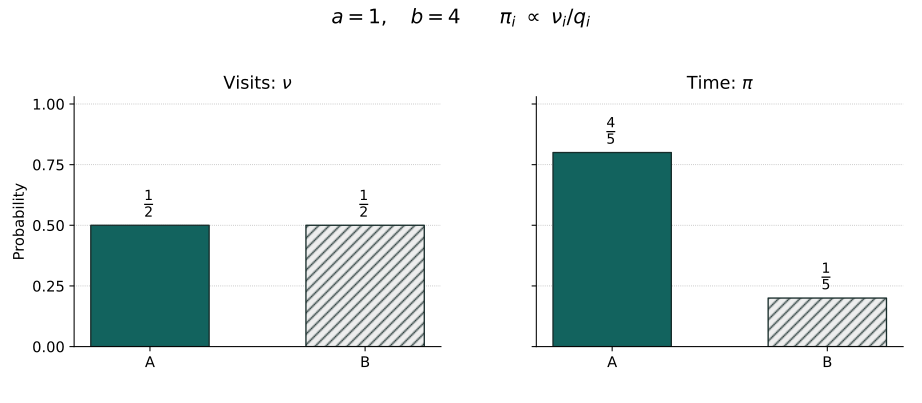
Equal visits need not mean equal time. Let A be working and B repair, with a=1,b=4. The left-hand halves come from alternating embedded visits; the right-hand four-fifths and one-fifth are proved stationary time weights from mean holds1 and1/4. They are not empirical frequencies of a finite simulation, and the figure does not prove convergence. Hatching and shading distinguish states in monochrome. The vector PDF shares exact parameters with the SVG.

22.15 Why continuous time removes a finite chain’s periodic obstruction

For finite irreducible Q, choose c>maxqᵢ so the uniformized matrix R=I+Q/c has positive diagonal entries. R is irreducible and aperiodic. Chapter 17 proved that Rⁿ converges to its unique invariant probability π. This π satisfies πQ=0 and is invariant for the continuous chain.

Given ε>0, choose K so every discrete distance for n≥K is below ε. The remaining finite part is bounded by P(Poisson(ct)<K), which vanishes as t→∞. Continuous time does not make the actual embedded chain aperiodic; it randomizes the number of observed steps, with virtual self-steps yielding an aperiodic matrix. Even an alternating embedded chain gives a unique large-time equilibrium. This does not replace general Harris or stronger mixing theory.

22.16 A separate clock for each individual: the Yule process

Take λ>0 and let each individual independently give birth at rate λ, remaining alive afterward. With n individuals, exponential competition makes the next birth wait Exp(λn), with a uniformly chosen parent. The population Zₜ is a pure-birth chain with λₙ=λn. Section9’s harmonic criterion guarantees that infinitely many births cannot occur in finite time. Below Zₜ consistently denotes population.

Starting at1, the forward integral equation closes successively in n. We have p₁(t)=e^(−λt), and for n≥2, pₙ′=λ(n−1)pₙ₋₁−λnpₙ with pₙ(0)=0. Each state has only one incoming state, so no infinite-column exchange is needed. Induction by integrating factors, or substitution plus this successive uniqueness, gives:

The masses sum to1; moments follow by differentiating the geometric series. Construct descendants of z initial individuals independently and merge them. Exponential competition reproduces the same λn rule, so their total has the law of the pure-birth chain started at z. This establishes branching, rather than declaring family independence merely from linear population rates.

22.17 A population limit without borrowing future convergence theory

Branching and Markov properties give E(Zₜ|Fₛ)=Zₛe^(λ(t−s)), so Mₜ=e^(−λt)Zₜ is a martingale with EMₜ²=2−e^(−λt)≤2. Chapter 15’s discrete-time convergence theorem does not automatically cover every real time. This special model can instead be settled directly by Chapter 12’s random series.

Here Aₙ is the first time population reaches n, with A₁=0; the symbol Aₙ distinguishes it from the nth jump time Tₙ of Section2. The centered series has independent terms with summable variances Σ1/k², so Chapter 12’s proved series theorem gives almost sure convergence. The harmonic-logarithm difference converges by integral bounds and monotonicity. Therefore n e^(−λAₙ)→e^(−L)>0.

For Aₙ≤t<Aₙ₊₁, n e^(−λAₙ₊₁)≤Mₜ≤n e^(−λAₙ). Both bounds converge to e^(−L), since n/(n+1)→1. This proves convergence to W>0 along all real times on one event. The second-moment bound gives uniform integrability: E[Mₜ;Mₜ>K]≤EMₜ²/K≤2/K. Chapter 7’s Vitali criterion applied to every sequence tₘ→∞ gives L¹ convergence and EW=1.

The exact geometric tail identifies the limit law. Survival here is certain, but the eventual random proportion is not. A mean growth curve does not specify what fraction one family will realize. This example’s second moments and explicit clock prevent mean loss, without erasing Chapter 20’s L log L obstruction for general families.

22.18 A reproduction may bring many children, or none

More generally, take β>0 and let each individual live an independent Exp(β) time and is replaced at death by K children, where P(K=k)=pₖ, K is a finite nonnegative integer and m=EK<∞. Children repeat the rule independently. With population z, reproduction completions have total rate βz and a uniform parent, changing population by K−1. When K=1 the population stays unchanged although a life replacement occurs; the population chain’s real exit rate is therefore not βz.

To construct the timed family itself, invisible one-child events cannot simply be discarded. Add J to count every reproduction completion. From (z,j), jump to (z−1+k,j+1) at rate βzpₖ, with z=0 absorbing. For V(z,j)=z+j+1, sublevel sets are finite and each increment is k, so QV=βzm≤βmV. Section11 proves nonexplosion of all reproduction events, not merely visible population changes.

At each event independently choose a uniform parent and attach finitely numbered children to the genealogy. Bounded time has finitely many events, each with finitely many children, giving a countable tree with defined birth and death times. Exponential competition and memorylessness identify this with assigning independent lifetimes and offspring numbers to individuals. Independent product constructions for distinct initial ancestors establish branching probabilistically.

The correspondence between independent lifetimes and uniform parent choice can be checked directly. For z independent Exp(β) clocks, specify clock i as first at s and require all other residual lifetimes to exceed rⱼ. The joint probability density is βe^(−βzs)∏ⱼ≠ᵢe^(−βrⱼ)ds. Dividing by the marginal density for first time and index restores independent Exp(β) residuals, independently of that time and index. Add fresh independent clocks for newborns and induct over events to align the two constructions exactly. This makes no claim of uniform parent choice for arbitrarily correlated clocks.

22.19 Generational fate and temporal speed require separate calculations

Suppressing lifetimes gives Chapter 20’s Galton–Watson tree, whose extinction probability is the least fixed point of f(s)=EKˢ. Nonexplosion identifies the two extinction events: a genealogy terminating in a finite generation contains finitely many individuals with finite lifetimes and reaches population0 in finite time. A genealogy surviving every generation cannot hit0 at a finite time and later produce descendants. This makes no claim about general continuous-state branching.

The temporal mean needs a separate calculation. The stopped V estimate and Fatou give E(Zₜ+Jₜ+1)≤(z+1)e^(βmt), ensuring locally finite population means. Starting with one ancestor, put u(t)=EZₜ. If its first lifetime exceeds t there is one individual; if it ends at s≤t it leaves on average m independent subfamilies of age t−s. Nonnegative Fubini gives:

Multiply by e^(βt) to obtain v(t)=1+βm∫₀ᵗv(r)dr. Local integrability first yields continuity, then differentiability, solving v′=βmv with v(0)=1. Branching now makes e^(−β(m−1)t)Zₜ a martingale. If m>1 and p₀>0, exponential mean growth coexists with positive extinction probability. If p₁=1, the family survives forever with population constantly1 while life-replacement events continue.

Normalized limits, L log L boundaries and diffusion limits for general continuous-time branching do not follow from this mean formula. We have constructed the finite-mean discrete-offspring exponential-lifetime model, proved nonexplosion, extinction identification and its mean martingale, and obtained the complete explicit Yule limit. Proof responsibility for more general normalized limits, L log L boundaries and diffusion approximations remains unassigned. Chapter 58 concerns multifurcating CRTs and mass splits; it is not a proof location for general continuous-time branching theory.

22.20 What lies between a matrix and a path?

The original machine needed only two clocks. Extending the same local description to infinitely many states exposed a hidden boundary: individually valid next steps can exhaust infinitely many steps in finite time. A rate matrix specifies local change, minimal construction determines how far it runs, and nonexplosion extends the rule through the whole future.

The two Kolmogorov equations are therefore more than two orders of matrix multiplication. They organize paths by first and last jumps, demanding different controls on infinite sums. Invariance distinguishes visit-sampled from time-sampled worlds, while the Yule family shows that a tree placed in real time still needs a proof of its random growth proportion.

Between jumps a path stands still. If changes become finer, with more numerous and smaller fluctuations in short intervals, valid individual changes still cannot replace proofs of path existence and path limits. We have learned not to mistake a local rule for a whole future. The next exploration carries that distinction to continuous paths.

Historical sources, proof provenance and scope

Kolmogorov’s 1931 paper Über die analytischen Methoden in der Wahrscheinlichkeitsrechnung, Mathematische Annalen104,415–458, is an original source on analytical methods for random evolution. Our countable-product construction, cemetery convention and jump expansion are modern reconstructions, not claims to reproduce the paper’s original presentation.

Yule’s original A Mathematical Theory of Evolution studies growth of species and genera, in Philosophical Transactions B213,21–87, conventionally catalogued as1925; the scan also retains a1924 separate-publication date. We reconstruct the linear birth mechanism as a population model with independent exponential clocks, without treating its biological assumptions as universal or conflating volume year and separate-publication date.

The technical scope can be compared with Norris’s institutional contents and section on forward and backward equations. We supply our own proofs rather than reproduce its exposition. For unbounded rates the forward equation is proved in integral and almost-everywhere differential form, and pointwise for bounded columns. General-state jump kernels, infinite activity, general boundary classification, Harris theory and continuous-state branching are not counted as completed here.

Direct prerequisites are independent random series, discrete stopping and information, Markov structure, branching families, and exponential clocks and the Poisson process. Measure uniqueness and monotone classes are available in the complete companion proof.