Haobai Wang · Public reading edition · ch06-en-7220fb2c8b05
This content fingerprint identifies the text, not academic final approval or an independent proof of authorship.
SHA-256: 7220fb2c8b0555cfdc9825fa9b3ec10a47ea5f6365e27c7f2b36ff13a10be16b
The Mathematics of Chance
Volume II · Probability in an Infinite World
Chapter 6: The Rebirth of the Average—From Weighted Sums to the Lebesgue Integral
Why should a simple average of gambling winnings ultimately require an entirely new theory of integration?
In Chapter 5, we underwent a major transformation in mathematical thought.
To define probability on infinite sets, we had to abandon a seemingly natural wish: not every set can have a measure compatible with interval length.
We therefore established the probability space
(\Omega,\mathcal F,P).Probability became more than “the number of favorable outcomes divided by the total number of outcomes”: it became a countably additive measure defined on a \sigma-algebra.
This finally enabled us to study continuous distributions, infinite random sequences, and complicated random objects such as Brownian motion rigorously.
Looking back over the development of probability, however, we find another mathematical concept of almost equal importance that has accompanied us throughout.
It is expectation.
In Chapter 1, we used expectation to divide the stakes fairly in an unfinished game.
In Chapter 2, we used expectation to estimate unknown parameters.
In Chapter 3, we used means and variances to study normal limits.
In Chapter 4, we even calculated the expectation of the sum of squared increments of an entire stochastic process.
But we never really answered:
Why should expectation be defined in the familiar way? What exactly is expectation when the sample space is no longer finite?
We now possess measure.
Perhaps it is time to understand averages afresh, from the beginning.
6.1 It Still Begins with a Fair Game of Chance
Imagine returning once more to Chapter 1.
A gambling contract has three possible payoffs:
X=
\begin{cases}
10,&\text{with probability }1/2,\\
20,&\text{with probability }1/3,\\
-5,&\text{with probability }1/6.
\end{cases}
If we want a single number to represent its average payoff, the most natural calculation is
\begin{aligned}
\mathbb E[X]
&=10\cdot\frac12
+20\cdot\frac13
-5\cdot\frac16\\
&=\frac{65}{6}.
\end{aligned}
Here we are taking a weighted sum:
\boxed{
\mathbb E[X]=\sum_i x_ip_i.
}
But we should examine this expression more closely.
It actually contains two entirely different mathematical objects.
The first is the payoff:
x_i.The second is the probability weight associated with each payoff:
p_i.Expectation is a mathematical operation combining the two.
Now write it in another form.
Let the sample space be
\Omega=\{\omega_1,\omega_2,\omega_3\},and define the random variable
X(\omega_1)=10,\quad
X(\omega_2)=20,\quad
X(\omega_3)=-5.
with corresponding probabilities
P(\{\omega_1\})=\frac12,\quad
P(\{\omega_2\})=\frac13,\quad
P(\{\omega_3\})=\frac16.
Then
\mathbb E[X]
=
\sum_{\omega\in\Omega}
X(\omega)P(\{\omega\}).
This formula already comes very close to the idea of integration.
What we are doing, in fact, is:
Accumulating the values of a function on the sample space, weighted according to a rule for the sizes of sets.
A new question therefore arises:
If the sample space has infinitely many outcomes, can this weighted summation be extended to some kind of integral?
6.1.1 From Finite to Continuous Outcomes
Suppose the payoff is no longer restricted to three values.
From [0,1], we choose a real number U uniformly at random, then receive the payoff
X=U^2.Chapter 5 has already supplied a rigorous uniform probability space:
\Omega=[0,1],
\qquad P=\text{Lebesgue length measure}.
We want to calculate
\mathbb E[U^2].From calculus, we would naturally write:
\mathbb E[U^2]
=
\int_0^1x^2\,dx
=
\frac13.
But this step contains an assumption we have not yet explained:
Why should the average of a continuous random variable equal an area integral of a function over an interval?
Our usual explanation is that the interval can be divided into many small pieces.
For example:
0=x_0<x_1<\cdots<x_n=1.For each small interval
I_k=[x_{k-1},x_k],choose a representative point \xi_k.
The expectation then appears to be approximated by
\sum_{k=1}^n\xi_k^2P(U\in I_k).Since U is uniformly distributed,
P(U\in I_k)=x_k-x_{k-1}.Hence
\mathbb E[U^2]
\approx
\sum_{k=1}^n\xi_k^2(x_k-x_{k-1}).
As the mesh becomes finer, this becomes the Riemann integral.
\boxed{
\mathbb E[U^2]
=
\int_0^1x^2\,dx.
}
This seems to suggest that we need no new theory of integration at all.
If calculus already provides the Riemann integral, why not simply apply it to every random variable?
The answer is that the Riemann integral depends on a particular method of approximation.
When we begin studying truly complicated random events and functions, that method encounters insurmountable difficulties.
6.2 What, Exactly, Does the Riemann Integral Do?
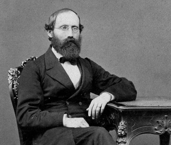
Bernhard Riemann(1826—1866)
A German mathematician. In his 1854 study of integration, he systematically investigated when functions more general than continuous functions could be integrated; the work was published in 1867.
Later, in 1875, Darboux developed the classical formulation of Riemann integrability in terms of upper and lower sums.
The intuitive idea behind the Riemann integral is very simple.
Given a function
f:[a,b]\to\mathbb R.we want to calculate the signed area beneath its graph.
To do so, we divide the horizontal axis into small intervals and approximate the graph with rectangles.
The Riemann integral: partition the domain first
The rectangles’ widths come from the partition of the domain, while their heights are determined by the function values on the respective intervals.
Define a partition
\mathcal P=\{a=x_0<x_1<\cdots<x_n=b\}.For a bounded function f, set
m_k=\inf_{x\in[x_{k-1},x_k]}f(x),M_k=\sup_{x\in[x_{k-1},x_k]}f(x).The lower and upper sums are, respectively,
L(f,\mathcal P)=
\sum_{k=1}^nm_k(x_k-x_{k-1}),
U(f,\mathcal P)=
\sum_{k=1}^nM_k(x_k-x_{k-1}).If we can make
U(f,\mathcal P)-L(f,\mathcal P)arbitrarily small, then f is Riemann integrable.
Behind this definition lies an important requirement:
As we divide the horizontal axis more finely, we must be able to control the function’s oscillation within the small intervals sufficiently well.
For continuous functions, this is of course no problem.
A continuous function on a compact interval is uniformly continuous.
But what about a function discontinuous everywhere?
Then things change.
6.2.1 A Function Entirely Natural in Probability That Cannot Be Riemann Integrated
Return to Chapter 5.
We already know that when choosing a real number uniformly on [0,1],
P(U\in\mathbb Q)=0.Now define
f(x)=\mathbf1_{\mathbb Q\cap[0,1]}(x).In other words:
f(x)=
\begin{cases}
1,&x\in\mathbb Q,\\
0,&x\notin\mathbb Q.
\end{cases}
This is usually called the Dirichlet function.
From a probabilistic viewpoint, it is entirely ordinary.
It simply represents the event
A=\{U\in\mathbb Q\}through its indicator function.
We want its expectation to equal the probability of that event:
\mathbb E[\mathbf1_A]=P(A)=0.But what happens if we try to use the Riemann integral?
Consider any partition
\mathcal P=\{0=x_0<\cdots<x_n=1\}.Since every nondegenerate subinterval contains both rational and irrational numbers,
m_k=0,\qquad M_k=1.we have
L(f,\mathcal P)=0,while
U(f,\mathcal P)=1.However fine the mesh,
\boxed{
U(f,\mathcal P)-L(f,\mathcal P)=1.
}
Thus f is not Riemann integrable.
We have encountered a real problem.
Probabilistically, the expectation of this random variable could hardly be clearer:
\mathbb E[f(U)]=0.Yet the traditional Riemann integral cannot assign it an integral value.
We cannot simply dismiss this function as “too irregular to be worth studying.”
Indicators of events are the most basic random variables in probability theory.
An integration theory that cannot generally handle indicators of measurable events cannot provide a complete foundation for expectation in modern probability.
We therefore need a new method of integration.
6.3 Lebesgue’s Change of View: Partition Values Before Positions
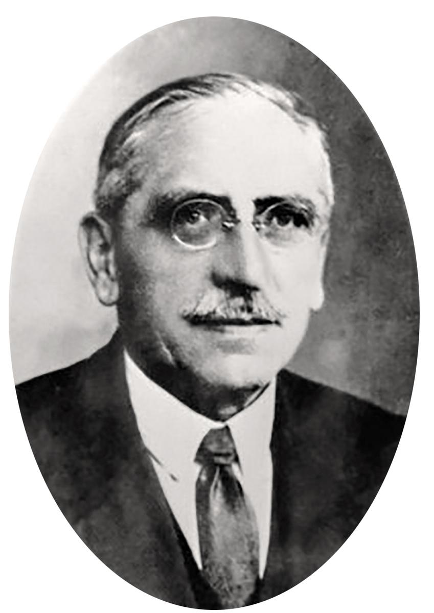
Henri Lebesgue(1875—1941)
A French mathematician.
In 1901, Lebesgue published a short paper on extending integration; in his 1902 doctoral dissertation, Intégrale, longueur, aire (Integral, Length, Area), he systematically developed new methods of measure and integration.
Lebesgue’s breakthrough did more than make certain previously nonintegrable functions integrable.
More fundamentally, he changed how we organize integration.〔55, 56〕
Riemann’s method can be understood as:
First divide the domain into small pieces, then examine the function values on each piece.
Lebesgue integration lets us organize the problem in the opposite direction:
First consider the values a function can take, then ask how large the sets of points having those values are.
Suppose a function f takes only three distinct values:
f(x)=
\begin{cases}
1,&x\in A_1,\\
3,&x\in A_2,\\
5,&x\in A_3,
\end{cases}
where
[0,1]=A_1\sqcup A_2\sqcup A_3.Assume these sets are all measurable.
Instead of dividing the horizontal axis into ever more small intervals, we can ask directly:
How large is the set where the function equals 1?
Where it equals 3?
Where it equals 5?
We naturally obtain
\boxed{
\int f\,dm
=
1\cdot m(A_1)
+3\cdot m(A_2)
+5\cdot m(A_3).
}
Is this not the weighted average with which we began?
The weights are now the measures of the sets corresponding to each function value, rather than the probabilities of three discrete outcomes.
Now reconsider the Dirichlet function.
f=\mathbf1_{\mathbb Q\cap[0,1]}.It takes only two values:
0,\qquad1.The set where it equals 1 is
\mathbb Q\cap[0,1],and its Lebesgue measure is 0.
The set where it equals 0 is the irrational part, whose measure is 1.
Thus:
\begin{aligned}
\int_0^1f\,dm
&=
1\cdot m(\mathbb Q\cap[0,1])\\
&\quad+
0\cdot m([0,1]\setminus\mathbb Q)\\
&=0.
\end{aligned}
The problem is solved.
There is a subtle distinction here.
We did not change the function itself.
Nor did we find a way to make it continuous.
We changed how we measure and accumulate its values.
A function may fluctuate with extreme irregularity across its domain while still having a very simple structure in terms of measure.
This is one of the most important changes of viewpoint in Lebesgue integration.
So far, however, we have handled only functions taking finitely many values.
The real difficulty is:
What should we do when a function takes infinitely many values?
6.4 Begin with the Simplest Functions: Integration Is Weighted Summation
In Chapter 5, we discovered an important method.
When we cannot directly measure arbitrarily complicated sets, we can begin with intervals and extend to more general sets through suitable limiting procedures.
We now apply a similar method to functions.
Do not try to integrate arbitrarily complicated measurable functions from the outset.
Study the simplest functions first, then gradually extend the reach of integration.
6.4.1 The Birth of Simple Functions
Let (\Omega,\mathcal F,\mu) be a measure space.
Consider a function
s:\Omega\to[0,\infty)and suppose it takes only finitely many distinct values:
a_1,\ldots,a_m.If every set
A_i=\{\omega:s(\omega)=a_i\}is measurable, we can write
\boxed{
s=\sum_{i=1}^ma_i\mathbf1_{A_i}.
}
Such a function is called a nonnegative simple function.
Notice that we have not required the sets A_i to be intervals.
They may be complicated Borel sets, measurable subsets of the Cantor set, or events in a general probability space.
Because these sets are pairwise disjoint, we can naturally define:
\boxed{
\int_\Omega s\,d\mu
=
\sum_{i=1}^ma_i\mu(A_i).
}
When a_i=0, the corresponding term is defined to be 0, even if \mu(A_i)=\infty.
This is the integral of a simple function.
If \mu=P is a probability measure, it returns exactly to the expectation formula from Chapter 1:
\mathbb E[s]
=
\sum_{i=1}^ma_iP(A_i).
We can see:
Lebesgue integration begins by extending finite weighted summation to measurable sets, rather than by introducing an entirely unfamiliar operation.
It preserves all our earlier basic intuitions about expectation.
For example, for nonnegative simple functions s,t and constants a,b\ge0,
\int(as+bt)\,d\mu
=
a\int s\,d\mu+b\int t\,d\mu.
Why?
Using the sets on which s,t take their respective values, we can construct a common finite measurable partition.
On each part, both functions are constant, so the equality above follows simply from distributivity of finite sums and finite additivity of measure.
Likewise, if
0\le s\le t,then
\int s\,d\mu\le\int t\,d\mu.All these properties are natural for simple functions.
The real question is how to proceed from simple functions to general measurable functions.
6.4.2 Why Can Every Nonnegative Measurable Function Be Approximated by Simple Functions?
Suppose
f:\Omega\to[0,\infty]is a nonnegative measurable function.
We want a sequence of simple functions
s_1,s_2,\ldotssuch that
0\le s_1\le s_2\le\cdotsand
s_n(\omega)\uparrow f(\omega)for every \omega.
Can this be done?
A natural idea is to divide the axis of function values into increasingly small intervals.
For example, use intervals of length 1/2 on the first step.
Use intervals of length 1/4 on the second.
At step n, use intervals of length 2^{-n}.
Then round each function value down to the nearest grid point.
To ensure finitely many values at every step, also truncate the function at n.
Define
\boxed{
s_n(\omega)
=
2^{-n}\left\lfloor
2^n\min\{f(\omega),n\}
\right\rfloor.
}
Here f(\omega)=\infty is permitted.
The expression may look complicated, but its meaning is simple:
First, disregard function values beyond n.
Then approximate the remaining part from below with precision 2^{-n}.
For every n, s_n takes only finitely many values and is therefore simple.
Because f is measurable, each of its level sets is measurable too.
Moreover, as n increases, the truncation level rises and the mesh becomes finer, so
s_n\le s_{n+1}.Finally,
\boxed{s_n(\omega)\uparrow f(\omega).}We have obtained an important construction theorem:
Every nonnegative measurable function can be approximated pointwise by a monotonically increasing sequence of nonnegative simple functions.
This step is one of the foundations of Lebesgue integration.
It tells us that however complicated the values and variations of f may be, we can still approximate it progressively through finite weighted summation.
6.4.3 If We Can Approximate, Why Not Define the Integral Directly?
We now know how to integrate simple functions.
And every nonnegative measurable function can be approximated from below by simple functions.
A very natural idea therefore arises:
Collect the integrals of all simple functions lying below f, then take their supremum.
Thus define
\boxed{
\int_\Omega f\,d\mu
=
\sup\left\{
\int_\Omega s\,d\mu:
0\le s\le f,\ s\text{ is a simple function}
\right\}.
}
This is the Lebesgue integral of a nonnegative measurable function.
Its value may at this stage be +\infty.
But this is no defect in the definition.
It is an outcome the theory deliberately permits.
We do not yet require every random variable to have a finite expectation, since that would force us to exclude many natural probability models.
Now look again at this definition.
It extends the familiar finite weighted sum:
\sum_{i=1}^ma_i\mu(A_i)to general measurable functions:
\int f\,d\mu.It uses no continuity of the function, requires no density, and does not even require \Omega to be an interval of real numbers.
It can therefore handle random variables, random functions, and measurable objects on even more abstract spaces.
But now a truly important difficulty appears.
We know that s_n\uparrow f.
May we conclude:
\int s_n\,d\mu\longrightarrow\int f\,d\mu?Only if the answer is yes does our entire approach of approximating general functions by simple functions truly work.
This is the problem solved by the monotone convergence theorem.
6.5 Beppo Levi: Why Does Approximation from Below Lose No Integral?
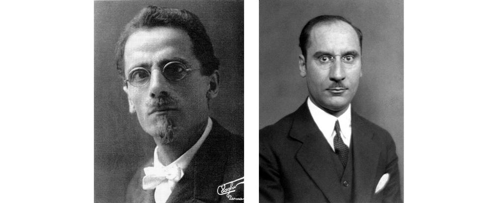
Beppo Levi(1875—1961)
An Italian mathematician. The important convergence result he proved in 1906 is now usually called Beppo Levi’s theorem or the monotone convergence theorem.
There is a historical detail worth noticing here.
Modern measure-theory textbooks often teach the “monotone convergence theorem, Fatou’s lemma, dominated convergence theorem” in that order.
The historical sequence was not quite the same. Lebesgue’s 1902 dissertation already contained the idea of bounded convergence, while Beppo Levi and Fatou made important contributions in 1906; more general forms of dominated convergence developed in Lebesgue’s later work.〔57〕
We shall continue by following the natural mathematical questions.
Theorem 6.1: Monotone Convergence Theorem
Editorial supplement: The limit function
fis also assumed nonnegative and measurable; on an incomplete space, almost everywhere convergence should be interpreted using a measurable version of the limit. See Appendix E. A proof from simple integrals without assuming general linearity is given in the monotone-convergence companion.
Let f_1,f_2,\ldots be nonnegative measurable functions satisfying
0\le f_1\le f_2\le\cdotsand
f_n(\omega)\uparrow f(\omega)almost everywhere.
Then
\boxed{
\lim_{n\to\infty}
\int_\Omega f_n\,d\mu
=
\int_\Omega f\,d\mu.
}
Both sides are permitted to equal +\infty.
This theorem is exceptionally powerful.
It does not require \mu(\Omega) to be finite.
It does not require a uniform upper bound on the f_n.
It does not even require their integrals to be finite.
It requires only nonnegativity and monotone increase.
Why are these two conditions so effective?
6.5.1 Proof: First Understand the Easy Direction
Since
f_n\le f,monotonicity of the integral gives
\int f_n\,d\mu\le\int f\,d\mu.Hence
\lim_{n\to\infty}\int f_n\,d\mu
\le
\int f\,d\mu.
This part presents no difficulty.
The real issue is the reverse direction:
\int f\,d\mu
\le
\lim_{n\to\infty}\int f_n\,d\mu.
We must prove:
Although the f_n always lie below f, their integrals cannot permanently miss some part of f.
6.5.2 The Key to the Proof: Compare with an Arbitrary Simple Function
Take any nonnegative simple function s satisfying
s\le f.We want to prove
\int s\,d\mu
\le
\lim_{n\to\infty}\int f_n\,d\mu.
If this holds for every such s, taking the supremum over s gives the result.
But we cannot simply assert that for some sufficiently large n we must have f_n\ge s.
The functions f_n may keep approaching f from below without ever reaching portions of s=f exactly.
To get around this, introduce a slightly smaller factor.
Take any
0<c<1.Define
A_n=\{\omega:f_n(\omega)\ge c\,s(\omega)\}.Because f_n\uparrow f and s\le f, we can show
A_n\uparrow\Omegaon the set where pointwise convergence holds.
Indeed, if s(\omega)>0, then
f(\omega)\ge s(\omega)>c\,s(\omega),Thus, for sufficiently large n,
f_n(\omega)\ge c\,s(\omega).If s(\omega)=0, then because f_n\ge0, this inequality holds for every n.
Hence
f_n\ge c\,s\mathbf1_{A_n}.By monotonicity of the integral,
\int f_n\,d\mu
\ge
c\int s\mathbf1_{A_n}\,d\mu.
Since s is simple, we can write
s=\sum_{j=1}^ma_j\mathbf1_{E_j}.Thus
\int s\mathbf1_{A_n}\,d\mu
=
\sum_{j=1}^ma_j\mu(E_j\cap A_n).
Because
E_j\cap A_n\uparrow E_jholds after removing a null set, and Chapter 5 established continuity of measure along increasing sequences of sets,
\mu(E_j\cap A_n)\uparrow\mu(E_j).Therefore
\lim_{n\to\infty}
\int s\mathbf1_{A_n}\,d\mu
=
\int s\,d\mu.
Hence
\lim_{n\to\infty}\int f_n\,d\mu
\ge c\int s\,d\mu.
Letting c\uparrow1 gives
\lim_{n\to\infty}\int f_n\,d\mu
\ge\int s\,d\mu.
This holds for every simple function satisfying 0\le s\le f.
Taking the supremum therefore gives:
\lim_{n\to\infty}\int f_n\,d\mu
\ge
\sup_{0\le s\le f}
\int s\,d\mu
=
\int f\,d\mu.
Combining the two directions,
\boxed{
\int f_n\,d\mu\uparrow\int f\,d\mu.
}
This completes the proof.
6.5.3 What Does This Theorem Really Reveal?
I believe the most memorable feature here is more than the auxiliary set A_n used in the proof.
It is a deeper principle:
We can recover the integral of a nonnegative function by continually adding known information and improving approximations from below, without losing any positive contribution to the integral.
In Chapter 5, we saw that probability measures satisfy
A_n\uparrow A
\implies P(A_n)\uparrow P(A).
Now, in Chapter 6, we find the corresponding statement for functions:
f_n\uparrow f
\implies
\int f_n\,dP\uparrow\int f\,dP.
The connection is entirely natural.
Indeed, choosing
f_n=\mathbf1_{A_n},gives
\int f_n\,dP=P(A_n).Continuity of measure from below can therefore be viewed as the monotone convergence theorem applied to indicator functions.
Conversely, the monotone convergence theorem extends this continuity from sets to general nonnegative measurable functions.
This is precisely the unity we have been seeking:
\boxed{
\text{limits of sets}
\quad\longrightarrow\quad
\text{limits of functions}
}
Probability and integration are no longer two unrelated theories.
Integration is the natural extension of the idea of measure to functions.
6.6 A New Difficulty: Not Every Random Variable Has a Finite Expectation
So far, we have discussed only nonnegative measurable functions.
Gambling payoffs, however, can be negative.
Random variables in the real world can also take both positive and negative values.
How should we define their integrals?
The most natural method is to separate a real-valued function into its positive and negative parts.
Define
f^+=\max\{f,0\},f^-=\max\{-f,0\}.Then
f=f^+-f^-,and
|f|=f^++f^-.Since f^+,f^- are both nonnegative measurable functions, we already know how to define their integrals.
We therefore try defining
\boxed{
\int f\,d\mu
=
\int f^+\,d\mu-\int f^-\,d\mu.
}
But there is a problem.
If
\int f^+\,d\mu=\infty,
\qquad
\int f^-\,d\mu=\infty,
we obtain
\infty-\infty.This expression has no well-defined mathematical meaning.
We must therefore require at least one of the two integrals to be finite before defining their difference as an extended-real integral.
If we further require
\int|f|\,d\mu<\infty,then both integrals of f^+,f^- are finite.
We say that f is integrable.
On a probability space, this corresponds to
\boxed{
\mathbb E[|X|]<\infty.
}
It ensures that \mathbb E[X] is a finite real number.
6.6.1 A Game with Finite Payoffs but Infinite Expectation
Consider a new game of chance.
A player uses some randomizing device and receives a random payoff X.
Suppose
P(X=2^n)=2^{-n},
\qquad n=1,2,\ldots.
This is a valid probability distribution because
\sum_{n=1}^{\infty}2^{-n}=1.Moreover, X takes a finite value in every actual trial.
In other words,
P(X<\infty)=1.But calculating its expectation gives:
\begin{aligned}
\mathbb E[X]
&=\sum_{n=1}^{\infty}2^nP(X=2^n)\\
&=\sum_{n=1}^{\infty}2^n2^{-n}\\
&=\sum_{n=1}^{\infty}1\\
&=\infty.
\end{aligned}
Thus
\boxed{
X<\infty\text{ a.s.},
\qquad
\mathbb E[X]=\infty.
}
Every actual game pays only a finite amount, yet its theoretical average payoff is infinite.
This has the same basic structure as the famous St. Petersburg paradox.
It forces us to distinguish anew:
A random variable’s being almost surely finite and its having a finite expectation are different matters.
Furthermore, an infinite expectation does not mean that a person should be willing to pay any entrance fee, however high. Real decisions also involve wealth constraints, utility, risk, and ability to pay.
The “fair value” we used in Chapter 1 corresponds to mathematical expectation under specific pricing assumptions. It does not automatically equal everyone’s subjective valuation when facing risk.
6.6.2 Why Does the Cauchy Distribution Have No Expectation?
In Chapter 3, we encountered the standard Cauchy distribution:
f(x)=\frac1{\pi(1+x^2)}.Because the density is symmetric about the origin, one might immediately conclude
\mathbb E[X]=0.But this inference is dangerous.
We must examine the positive and negative parts separately.
For the positive part,
\begin{aligned}
\mathbb E[X^+]
&=\int_0^\infty\frac{x}{\pi(1+x^2)}\,dx\\
&=\frac1{2\pi}
\lim_{R\to\infty}\log(1+R^2)\\
&=\infty.
\end{aligned}
By symmetry,
\mathbb E[X^-]=\infty.Thus
\mathbb E[X]
=
\mathbb E[X^+]-\mathbb E[X^-]
is undefined.
Although the symmetrically truncated integrals satisfy
\lim_{R\to\infty}
\int_{-R}^{R}\frac{x}{\pi(1+x^2)}\,dx=0,
this is only the result of symmetric truncation in the sense of a Cauchy principal value, not an expectation in the Lebesgue sense.
We thereby learn:
Integration theory must tell us not only how to calculate an average, but also when an average does not exist at all.
This is the value of a rigorous definition.
6.7 Why Can We Not Freely Interchange Limits and Expectations?
We are finally ready to examine another of this chapter’s central questions.
Suppose we have a sequence of random variables
X_1,X_2,\ldotsand
X_n\longrightarrow Xalmost everywhere.
May we immediately conclude
\mathbb E[X_n]\longrightarrow\mathbb E[X]?This seems entirely reasonable.
If the values of the random variables are converging, why should their averages not converge as well?
Reality, however, is far less simple.
6.7.1 A Spike That Grows Narrower and Taller
Take Lebesgue measure on the interval [0,1] and define
f_n(x)=n\mathbf1_{(0,1/n)}(x).This function takes only two values:
f_n(x)=
\begin{cases}
n,&0<x<1/n,\\
0,&\text{elsewhere}.
\end{cases}
As n increases, the region where the function is nonzero narrows, while its height increases.
Shrinking-spike experiment: f_n=n\mathbf1_{(0,1/n)}. The nonzero interval has width 1/n and integral 1. The vertical axis uses a fixed scale for the selected n. The spike grows narrower, but its area always remains 1.
For any fixed x\in[0,1], eventually
f_n(x)=0.so
\boxed{f_n(x)\longrightarrow0}at every point.
Yet
\begin{aligned}
\int_0^1f_n(x)\,dx
&=
n\cdot\frac1n\\
&=1.
\end{aligned}
Thus
\boxed{
\lim_{n\to\infty}\int_0^1f_n(x)\,dx
=1
\ne
0
=
\int_0^1\lim_{n\to\infty}f_n(x)\,dx.
}
We do not even need complicated probability distributions here.
A sequence of very simple nonnegative functions already shows that pointwise convergence does not guarantee convergence of integrals.
What happened?
As n increases, the function’s entire contribution to the integral concentrates in an ever smaller region.
The spike eventually leaves every fixed point behind.
The pointwise limit therefore sees none of this contribution.
Yet the total area of each spike remains 1.
We may call this concentration of mass.
There is another, similar mechanism of failure.
On the whole real line, consider
g_n(x)=\mathbf1_{(n,n+1)}(x).Again,
g_n(x)\to0for every fixed x.
But
\int_{\mathbb R}g_n(x)\,dx=1.Here the mass does not concentrate in a shrinking interval.
It simply keeps moving toward infinity.
We may call this escape of mass.
We have therefore identified two reasons why limits of integrals can fail:
Excessive local concentration of mass, and mass escaping to infinity.
We now need a theorem that at least gives a universally valid estimate without demanding a complete interchange of limits and integrals.
This is Fatou’s lemma.
6.8 Fatou’s Lemma: What Can We Retain Even When Limits Cannot Be Interchanged?
Theorem 6.2: Fatou’s Lemma
Let f_1,f_2,\ldots be nonnegative measurable functions.
Then
\boxed{
\int_\Omega\liminf_{n\to\infty}f_n\,d\mu
\le
\liminf_{n\to\infty}\int_\Omega f_n\,d\mu.
}
We do not require f_n to be monotone.
We do not even require f_n itself to have a pointwise limit.
We use only the lower limit:
\liminf_{n\to\infty}f_n.The theorem can be understood as follows:
In a limiting sequence of nonnegative functions, contributions to the integral may disappear, but the integral of the lower-limit function cannot exceed the lower limit of the original integrals.
The spike example shows precisely how this inequality can be strict:
0<1.6.8.1 Why Does Fatou’s Lemma Follow from Monotone Convergence?
Define
h_n(\omega)=\inf_{k\ge n}f_k(\omega).Since we take infima over progressively smaller sets,
h_1\le h_2\le\cdots.and
h_n\uparrow\liminf_{n\to\infty}f_n.We may therefore apply the monotone convergence theorem:
\int\liminf_{n\to\infty}f_n\,d\mu
=
\lim_{n\to\infty}\int h_n\,d\mu.
On the other hand, for every k\ge n,
h_n\le f_k.so
\int h_n\,d\mu
\le
\inf_{k\ge n}\int f_k\,d\mu.
Letting n\to\infty gives
\begin{aligned}
\int\liminf_{n\to\infty}f_n\,d\mu
&=
\lim_n\int h_n\,d\mu\\
&\le
\lim_n\inf_{k\ge n}\int f_k\,d\mu\\
&=
\liminf_{n\to\infty}\int f_n\,d\mu.
\end{aligned}
This completes the proof.
This proof illustrates an important strategy in measure theory.
When the original sequence is not monotone, we can construct a new increasing sequence by taking infima over its tails.
The monotone convergence theorem can then solve a problem that was not initially monotone.
Fatou’s lemma is no magical rule completely independent of monotone convergence.
It develops naturally from that foundational structure.
But Fatou’s lemma still gives only a one-sided inequality.
To interchange integrals and limits fully, we must control the contributions that could concentrate or escape.
This leads us to one of the most frequently used theorems of Lebesgue integration.
6.9 The Dominated Convergence Theorem: What Can Prevent Integral Mass from Disappearing?
Reconsider the earlier counterexample:
f_n(x)=n\mathbf1_{(0,1/n)}(x).The problem is that although the function is nonzero only on a tiny region, its height becomes arbitrarily large as n increases.
If we could find a fixed integrable function g such that every f_n satisfies
|f_n|\le g,could we prevent this loss of control?
Indeed, this is the core of the dominated convergence theorem.
Theorem 6.3: Lebesgue’s Dominated Convergence Theorem
Editorial supplement: The limit function
fbelow is taken to be measurable; functions may be real or complex, with the proof interpreted componentwise as appropriate. See Appendix E. DCT holds on any measure space; see the integral foundations for nonnegative linearity, the common null set and the full proof.
Let f_n be a sequence of measurable functions, with
f_n\longrightarrow f
\qquad\mu\text{-a.e.}
Suppose there exists a nonnegative integrable function g such that
|f_n|\le g
\qquad\mu\text{-a.e.}
for every n.
Then f is integrable, and
\boxed{
\lim_{n\to\infty}\int f_n\,d\mu
=
\int f\,d\mu.
}
In fact, we obtain the stronger conclusion:
\boxed{
\int|f_n-f|\,d\mu\longrightarrow0.
}
This second conclusion shows that dominated convergence actually gives L^1 convergence, not merely convergence of the numerical integrals.
This will matter when we systematically study modes of random convergence.
6.9.1 Why Is an Integrable Upper Bound So Effective?
If
|f_n|\le gand
\int g\,d\mu<\infty,then for every measurable set A,
\int_A|f_n|\,d\mu
\le
\int_Ag\,d\mu.
Since g is integrable, its integral is absolutely continuous:
For any \varepsilon>0, there exists \delta>0 such that
\mu(A)<\delta
\implies
\int_Ag\,d\mu<\varepsilon.
Thus, however large n becomes, f_n cannot retain a fixed contribution to the integral in a region of arbitrarily small measure.
Likewise, an integrable dominator g has controlled tails. On a general measure space, finite-measure sets exhaust its effective support \{g>0\}, not necessarily the entire space. DCT itself requires no σ-finiteness; see the effective-support proof.
A fixed integrable upper bound therefore excludes exactly the uncontrolled integral mass present in our two earlier counterexamples.
This explains why dominated convergence requires an integrable dominating function, rather than simply some bound on function values.
For example, on an infinite-measure space,
|f_n|\le1need not suffice.
The earlier functions
g_n=\mathbf1_{(n,n+1)}all satisfy |g_n|\le1, yet we still cannot interchange limit and integral, because the constant function 1 is not integrable on the whole real line.
6.9.2 A Rigorous Proof of the Dominated Convergence Theorem
Now that we have Fatou’s lemma, the proof is quite concise.
Since
|f_n|\le gand f_n\to f almost everywhere,
|f|\le galmost everywhere.
Thus f is integrable.
Also,
g+f_n\ge0,
\qquad
g-f_n\ge0.
First apply Fatou’s lemma to the nonnegative functions g+f_n:
\int(g+f)\,d\mu
\le
\liminf_{n\to\infty}
\int(g+f_n)\,d\mu.
Because g is integrable, we may legitimately subtract \int g\,d\mu, obtaining
\boxed{
\int f\,d\mu
\le
\liminf_{n\to\infty}\int f_n\,d\mu.
}
Next apply Fatou’s lemma to g-f_n:
\int(g-f)\,d\mu
\le
\liminf_{n\to\infty}\int(g-f_n)\,d\mu.
Thus
\int g\,d\mu-\int f\,d\mu
\le
\int g\,d\mu-
\limsup_{n\to\infty}\int f_n\,d\mu.
Rearranging gives
\boxed{
\limsup_{n\to\infty}\int f_n\,d\mu
\le
\int f\,d\mu.
}
Combining the two inequalities:
\int f\,d\mu
\le
\liminf_n\int f_n\,d\mu
\le
\limsup_n\int f_n\,d\mu
\le
\int f\,d\mu.
Hence
\boxed{
\lim_{n\to\infty}\int f_n\,d\mu
=
\int f\,d\mu.
}
Finally, since
|f_n-f|\longrightarrow0almost everywhere, and
|f_n-f|\le2g,applying the integral-convergence conclusion just proved to the new sequence of nonnegative functions |f_n-f| gives
\boxed{
\int|f_n-f|\,d\mu\longrightarrow0.
}
This completes the proof.
6.9.3 The Relationship Among the Three Convergence Theorems
Let us review the three results we have established.
| Theorem | Essential conditions | Conclusion |
|---|---|---|
| Monotone convergence | 0\le f_n\uparrow f |
Integral and limit can be interchanged; infinite integrals are allowed |
| Fatou’s lemma | f_n\ge0 |
A one-sided inequality involving lower limits |
| Dominated convergence | f_n\to f a.e., |f_n|\le g\in L^1 |
Integrals converge, and f_n\to f in L^1 |
We see that these three theorems are not isolated pieces of knowledge.
They all answer the same question:
\boxed{
\text{When can a limit be moved inside an integral?}
}
We simply have different amounts of information for different sequences of functions.
If the functions increase monotonically, we can exploit approximation from below in the structure of the nonnegative integral.
If they are not monotone but remain nonnegative, Fatou’s lemma at least supplies a lower bound.
If they share an integrable dominating function, we can obtain full convergence.
This is a mathematical language of increasing precision.
The familiar order of these proofs primarily reflects modern mathematical logic, rather than the historical order of discovery. Beppo Levi, Fatou, Lebesgue, and Vitali made interconnected contributions to limits of integrals in the early twentieth century.〔57〕
6.10 Why Can Integration Unify the Distributions of All Random Variables?
We have now rigorously established the Lebesgue integral.
We can return to probability and resolve a question that has repeatedly arisen.
Suppose
X:(\Omega,\mathcal F,P)\to(\mathbb R,\mathcal B(\mathbb R))is a random variable.
We want to calculate
\mathbb E[h(X)]where h:\mathbb R\to\mathbb R is Borel measurable.
Must we know how X was constructed on the original sample space?
Not necessarily.
In fact, knowing the distribution of X suffices to calculate the expectations of all corresponding integrable functions.
6.10.1 Begin the Proof with Simple Functions
Recall Chapter 5:
P_X(B)=P(X^{-1}(B)).First consider a simple function:
h=\sum_{i=1}^ma_i\mathbf1_{B_i},where the B_i are Borel sets.
Then
h(X)
=
\sum_{i=1}^ma_i\mathbf1_{\{X\in B_i\}}.
Hence
\begin{aligned}
\mathbb E[h(X)]
&=\sum_{i=1}^ma_iP(X\in B_i)\\
&=\sum_{i=1}^ma_iP_X(B_i)\\
&=\int_{\mathbb R}h(x)\,P_X(dx).
\end{aligned}
For a nonnegative Borel measurable function h, choose a sequence of simple functions
h_n\uparrow h.Then apply the monotone convergence theorem to both sides to obtain
\boxed{
\mathbb E[h(X)]
=
\int_{\mathbb R}h(x)\,P_X(dx).
}
For general integrable h(X), extend the result using positive and negative parts.
This integral formula is often called the law of the unconscious statistician. Essentially, it is the change-of-variables formula for integration under a pushforward measure.
It tells us:
If we only want the expectation of a function of a random variable, we do not need to know the construction of the entire probability space behind it.
We need only its distribution measure P_X.
This is a remarkably powerful abstraction.
6.10.2 Discrete and Continuous Distributions Are Merely Special Cases
If X is discrete, taking values x_i with corresponding weights p_i, then
P_X=\sum_i p_i\delta_{x_i}.Here \delta_{x_i} is the Dirac measure concentrated at x_i.
Thus
\int h(x)\,P_X(dx)
=
\sum_i h(x_i)p_i.
We have returned to weighted summation.
If the distribution of X has a density f_X with respect to Lebesgue measure, then
P_X(dx)=f_X(x)\,dx.so
\int h(x)\,P_X(dx)
=
\int_{\mathbb R}h(x)f_X(x)\,dx.
We have returned to the familiar formula for continuous random variables.
Now, however, consider a more unusual random variable.
Suppose X has the Cantor distribution.
Its distribution function is continuous and it has no point atoms, yet its distribution is concentrated on the Cantor set, which has Lebesgue measure zero.
It is therefore neither discrete nor equipped with a probability density relative to Lebesgue measure.
Nevertheless,
\boxed{
\mathbb E[h(X)]
=
\int_{\mathbb R}h(x)\,P_X(dx)
}
remains perfectly valid.
We finally understand why modern probability should not define expectation as
\sum_xxf(x)or
\int xf(x)\,dx.since these cover only particular types of distributions.
The truly general form is
\boxed{
\mathbb E[X]
=
\int_\Omega X\,dP
=
\int_{\mathbb R}x\,P_X(dx),
}
provided that the relevant integral is defined.
This is entirely consistent with the outlook of the whole book.
We are not inventing a new theory unrelated to the old methods.
We have found a larger mathematical structure in which the old methods become special cases.
6.11 An Unexpected Formula: Expectation Can Also Be Calculated from Tail Probabilities
We already know that the expectation of a nonnegative random variable is
\mathbb E[X]=\int_\Omega X\,dP.But if we do not directly know the density of X and know only its tail probabilities
P(X>t),can we still calculate its expectation?
For a nonnegative real number x, there is a simple identity:
\boxed{
x=\int_0^\infty\mathbf1_{\{x>t\}}\,dt.
}
Why?
Because when x\ge0,
\mathbf1_{\{x>t\}}
=
\begin{cases}
1,&0\le t<x,\\
0,&t\ge x.
\end{cases}
so the right-hand side is simply the length of an interval of length x.
Replacing x with a nonnegative random variable X(\omega) gives
X(\omega)
=
\int_0^\infty\mathbf1_{\{X(\omega)>t\}}\,dt.
Hence
\mathbb E[X]
=
\int_\Omega
\left(
\int_0^\infty
\mathbf1_{\{X(\omega)>t\}}\,dt
\right)P(d\omega).
If we may interchange these two integrals, then
\begin{aligned}
\mathbb E[X]
&=
\int_0^\infty
\left(
\int_\Omega
\mathbf1_{\{X(\omega)>t\}}P(d\omega)
\right)dt\\
&=
\int_0^\infty P(X>t)\,dt.
\end{aligned}
Thus
\boxed{
\mathbb E[X]
=
\int_0^\infty P(X>t)\,dt.
}
This is sometimes called the tail integral formula or the layer-cake representation.
It reveals another interpretation of expectation:
The expectation of a nonnegative random variable can be understood as the accumulated probabilities of all its tail events.
For example, suppose
P(X>t)=e^{-\lambda t},
\qquad t\ge0.
Then
\mathbb E[X]
=
\int_0^\infty e^{-\lambda t}\,dt
=
\frac1\lambda.
Without first using a probability density, we obtained the expectation directly from tail probabilities.
This is especially important for heavy-tailed distributions.
If, for sufficiently large t,
P(X>t)\asymp t^{-\alpha},then the tail integral
\int_1^\infty t^{-\alpha}\,dtis finite if and only if \alpha>1.
Thus the rate of tail decay directly determines whether expectation is finite.
But our derivation left one question unresolved:
Why may we interchange the two integrals?
This leads us to the chapter’s final important theorem.
6.12 Fubini–Tonelli: When May We Change the Order of Summation and Integration?
Editorial supplement: Appendix C gives expanded proofs concerning sections of product sets, the monotone-class step, and the construction of product measure. The π–λ theorem and the set and functional monotone class theorems are proved fully in the generating-class companion.
Recall Chapter 1.
On finite probability spaces, we can freely change the order of finite summation:
\sum_{i=1}^m\sum_{j=1}^na_{ij}
=
\sum_{j=1}^n\sum_{i=1}^ma_{ij}.
This is an utterly ordinary algebraic property.
But when we study infinitely many random outcomes, may we still freely interchange sums and integrals?
Consider a random system with two components, whose outcome space is
\Omega_1\times\Omega_2.We want to take a function
f:\Omega_1\times\Omega_2\to\mathbb Rand calculate its integral.
We could integrate first in the second variable and then in the first.
Or we could reverse the order.
The question is:
\boxed{
\int_{\Omega_1}
\left(
\int_{\Omega_2}f(x,y)\,\nu(dy)
\right)\mu(dx)
\overset{?}{=}
\int_{\Omega_2}
\left(
\int_{\Omega_1}f(x,y)\,\mu(dx)
\right)\nu(dy).
}
Are these two expressions really equal in general?
To answer this, we must first understand product measure.
6.12.1 How Can We Assign Measure to the Joint Outcomes of Two Spaces?
Suppose
(\Omega_1,\mathcal F_1,\mu)and
(\Omega_2,\mathcal F_2,\nu)are two measure spaces.
For a rectangle
A\times B,the most natural definition is
(\mu\times\nu)(A\times B)=\mu(A)\nu(B).When \mu,\nu are probability measures, this agrees exactly with the multiplication rule for independent events.
Defining measure only on rectangles, however, is insufficient.
The joint space contains many sets that cannot be written as a single rectangle.
We therefore need the following \sigma-algebra generated by measurable rectangles:
\mathcal F_1\otimes\mathcal F_2
=
\sigma\{A\times B:A\in\mathcal F_1,B\in\mathcal F_2\}
and must construct a measure on it.
Under the assumption of \sigma-finiteness, measure extension theory constructs the unique product measure with the required values on rectangles.
Once again, this shows that the measure extension theory of Chapter 5 is far more than an isolated technical issue.
It allows us to construct rigorously, from individual random experiments, a joint space containing several experiments.
6.12.2 Tonelli’s Theorem: For Nonnegative Functions, Interchanging the Order Is Always Safe
Now suppose
f:\Omega_1\times\Omega_2\to[0,\infty]is a nonnegative product-measurable function, and both measure spaces are \sigma-finite.
Tonelli’s theorem tells us:
\boxed{
\begin{aligned}
\int_{\Omega_1\times\Omega_2}f\,d(\mu\times\nu)
&=
\int_{\Omega_1}
\left(\int_{\Omega_2}f(x,y)\,\nu(dy)\right)\mu(dx)\\
&=
\int_{\Omega_2}
\left(\int_{\Omega_1}f(x,y)\,\mu(dx)\right)\nu(dy).
\end{aligned}
}
The integrals are permitted to equal +\infty.
Let us first understand why this holds.
For the indicator of a rectangle,
f=\mathbf1_{A\times B},the conclusion is simply
(\mu\times\nu)(A\times B)=\mu(A)\nu(B).For nonnegative simple functions, linearity gives the corresponding formula.
Extending the result to general nonnegative measurable functions also requires a step concerning product-measurable sets and measurability of their sections. Start with rectangles and use a monotone-class argument to extend the integral identity to sets in the product \sigma-algebra, then to simple functions.
Finally, for any nonnegative measurable function f, choose simple functions
s_n\uparrow f,and apply the monotone convergence theorem successively to the relevant integrals.
This gives Tonelli’s formula.
Notice the structure.
The multiplicative relation between measures on rectangles is the starting point.
Simple functions turn it into finite weighted summation.
The monotone convergence theorem then extends the finite structure to arbitrary nonnegative measurable functions.
Tonelli’s theorem shows once more that Lebesgue integration draws its power from the interplay of simple objects, additivity of measure, and limiting operations.
The tail integral formula from Section 6.11 now has a rigorous justification too.
Since
(\omega,t)\longmapsto
\mathbf1_{\{X(\omega)>t\}}
is nonnegative and product measurable, Tonelli’s theorem lets us interchange the integrals without knowing beforehand that \mathbb E[X] is finite.
6.12.3 Fubini’s Theorem: With Both Signs Present, We Need More Conditions
For general real-valued functions, however, the situation differs.
If positive and negative contributions alternate infinitely, changing the order of integration may change the result or even make an integral undefined.
To understand the danger, begin with a wholly discrete example.
Define a doubly indexed sequence
a_{mn}=
\begin{cases}
1,&n=m,\\
-1,&n=m+1,\\
0,&\text{otherwise},
\end{cases}
\qquad m,n\ge1.
For every fixed m, the row contains exactly one 1 and one -1.
Thus
\sum_{n=1}^{\infty}a_{mn}=0.and hence
\boxed{
\sum_{m=1}^{\infty}
\left(\sum_{n=1}^{\infty}a_{mn}\right)=0.
}
But if we sum over m first:
The first column contains only a single 1, so its sum is 1.
For column n\ge2, there is exactly one 1 and one -1, so its sum is 0.
Thus
\boxed{
\sum_{n=1}^{\infty}
\left(\sum_{m=1}^{\infty}a_{mn}\right)=1.
}
We have obtained two different answers!
Why?
Because
\sum_{m,n}|a_{mn}|=\infty.the total absolute contribution of the positive and negative terms cannot be controlled.
Changing the order of infinite summation can therefore produce different results.
This reminds us:
The interchange property of finite sums cannot be extended without conditions to infinite sums or integrals.
We therefore need a more precise theorem.
Theorem 6.4: Fubini’s Theorem
Let f be a product-measurable real-valued function satisfying
\boxed{
\int_{\Omega_1\times\Omega_2}
|f|\,d(\mu\times\nu)<\infty.
}
Then the corresponding iterated integrals exist in the appropriate almost everywhere sense and satisfy
\boxed{
\begin{aligned}
\int_{\Omega_1\times\Omega_2}f\,d(\mu\times\nu)
&=
\int_{\Omega_1}
\left(\int_{\Omega_2}f(x,y)\,\nu(dy)\right)\mu(dx)\\
&=
\int_{\Omega_2}
\left(\int_{\Omega_1}f(x,y)\,\mu(dx)\right)\nu(dy).
\end{aligned}
}
The proof is now very natural.
Decompose f as
f=f^+-f^-.Since
f^+,f^-\le|f|,both of their integrals are finite.
Apply Tonelli’s theorem separately to the two nonnegative functions and subtract the results to obtain Fubini’s theorem.
We have finally found sufficient conditions for changing the order of integration.
Nonnegativity permits Tonelli’s theorem; absolute integrability permits Fubini’s theorem to handle positive and negative contributions safely.
These two theorems will recur throughout our later study of joint distributions, conditional expectation, stochastic integration, and stochastic processes.
6.13 From Fair Prices to Probabilistic Limits: What Have We Created?
We can now return to the gambling problem of Chapter 1.
There, expectation was simply a very elementary formula:
\mathbb E[X]=\sum_i x_ip_i.After this chapter, we finally understand the entire extensible mathematical structure behind that formula.
On finite spaces, we use weighted sums.
For simple functions, we extend the weights to measures of measurable sets.
For general nonnegative functions, we define integration through monotone approximation by simple functions.
For functions with both signs, we use positive and negative parts to define integrability.
We then study the conditions for interchanging integrals with limits, and integrals with other integrals.
This allows us to use the same expression on extraordinarily complicated probability spaces:
\boxed{
\mathbb E[X]=\int_\Omega X\,dP.
}
But I believe the real value of this formula goes beyond unifying discrete and continuous expectations.
It gives many seemingly different questions in probability the same logical structure.
For example, the law of large numbers studies random averages:
\frac1n\sum_{i=1}^nX_i.We need to know in what sense these averages converge.
Statistical inference studies sequences of estimators:
\widehat\theta_n.We need to know when limits can be used to estimate their risks:
\mathbb E[(\widehat\theta_n-\theta)^2].The theory of stochastic processes studies random variables evolving over time:
X_t.We need to know when limits and expectations can be interchanged:
\lim_{t\to t_0}\mathbb E[X_t]
\overset{?}{=}
\mathbb E\left[\lim_{t\to t_0}X_t\right].
Brownian motion, encountered in Chapter 4, likewise repeatedly requires this theory of integration and limits.
Lebesgue integration therefore does more than answer how to calculate an average.
One of its more important contributions is a stable mathematical language for analyzing limiting processes.
This makes an interesting comparison with our original understanding of expectation.
Initially, expectation told us how to value random payoffs that had not yet occurred.
Now it has become an integration operation on abstract function spaces.
It handles finite games of chance, but also continuous stochastic processes, singular distributions, random geometry, and infinite-dimensional probability models.
Chapter 6 Conclusion: Integration Is More Than Another Way to Calculate Area
Look back over the ideas of this chapter.
We began by wanting to extend finite weighted averages to continuous spaces.
It seemed we could simply use the Riemann integral.
But the Dirichlet function showed that this integral cannot handle certain elementary indicators of random events.
Instead of treating interval partitions of the domain as our only starting point, we therefore began with the sets corresponding to the values of measurable functions.
We defined the integral of a simple function:
\int s\,d\mu=\sum_i a_i\mu(A_i).Then, through approximation from below, extended it to general nonnegative measurable functions:
\int f\,d\mu
=
\sup_{0\le s\le f}
\int s\,d\mu.
Finally, positive and negative parts supplied the integral of a general integrable function.
But sequences of functions presented a new difficulty:
Even if
f_n\to fholds pointwise, it need not follow that
\int f_n\,d\mu\to\int f\,d\mu.We therefore needed the monotone convergence theorem, Fatou’s lemma, and the dominated convergence theorem.
To interchange two integrals, we also had to establish Tonelli’s and Fubini’s theorems.
A complete theory of integration gradually emerged.
Finite weighted averages
\sum_i a_ip_iIntegration of simple functions
\int\sum_i a_i\mathbf1_{A_i}\,d\muGeneral measurable functions
\int f\,d\mu=\sup_{0\le s\le f}\int s\,d\muExpectation in modern probability
\mathbb E[X]=\int_\Omega X\,dPNaturally connected with limit theorems, product measures, and stochastic processes
But there is one further question that I believe deserves deeper thought.
We have proved the dominated convergence theorem:
If X_n\to X almost everywhere, and
|X_n|\le Y,\qquad \mathbb E[Y]<\infty,then
\mathbb E[|X_n-X|]\to0.This shows that under suitable conditions, almost sure convergence implies L^1 convergence.
Yet we also saw the spike counterexample:
X_n\to0\quad\text{a.s.},which satisfies
\mathbb E[|X_n|]=1.Thus almost sure convergence alone does not imply L^1 convergence.
On the other hand, Chapter 2 discussed:
X_n\xrightarrow{P}X.Chapter 3 introduced:
X_n\xrightarrow{d}X.And Chapter 4 even studied:
X_n\Longrightarrow X
\quad\text{in }C([0,1]).
We seem to have acquired many mathematical expressions for “approaching the same random object,” without yet establishing their full connections.
The question therefore arises.
When we say that one sequence of random variables approaches another random variable, what exactly should we require?
Should their values approach one another along each sample path?
Should the probability of a deviation beyond a given threshold become smaller?
Or should only their probability distributions become increasingly similar?
Are these requirements equivalent?
If not, why do we need so many different notions of convergence?
This will mark another exceptionally important change of perspective.
Next Chapter: Chapter 7, “What Does Convergence Really Mean?—Four Kinds of Limits in a Random World”
We will begin with a seemingly counterintuitive question:
If the probability that an event occurs on trial
ntends to zero, why can it still occur infinitely often almost surely?
This question will take us back to the law of large numbers in Chapter 2 and reveal that decreasing probabilities and the eventual absence of exceptional behavior along a sample path are two different mathematical properties.
We will then gradually develop:
\boxed{
\begin{aligned}
&\text{Almost sure convergence},\\
&\text{Convergence in probability},\\
&L^p\text{ convergence},\\
&\text{Convergence in distribution}.
\end{aligned}
}
We will not merely state their relationships: rigorous counterexamples will show why each reverse implication can fail.
The Borel–Cantelli lemmas, the subsequence principle, uniform integrability, the Portmanteau theorem, and the idea of Skorokhod representation will gradually become natural parts of the story.
Ultimately, we hope to understand:
Convergence is not an isolated mathematical concept. Choosing a mode of convergence means deciding which kind of information about the random world we want to preserve.
The Mathematics of Chance · Volume II, Chapter 6 · Working draft v0.1