Six explanatory figure groups, with standalone print vectors. Only the typewriter example adds a new optional interaction. These figures aid the proofs; they do not replace them.
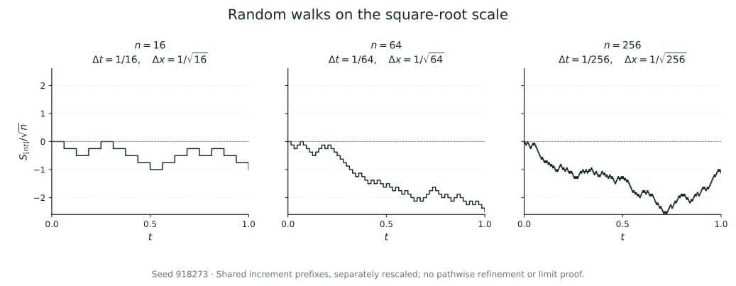
Smaller steps without vanishing fluctuations The time step is 1/n and the space step is 1/√n: approximately n steps per unit time preserve displacement variance 1. These are finite fixed-seed simulations using different prefixes of the same increment sequence, rescaled separately. They are not successive refinements of one path, do not show path-by-path convergence across n, and do not prove Donsker's theorem. The existing experiment lets you change the step count.
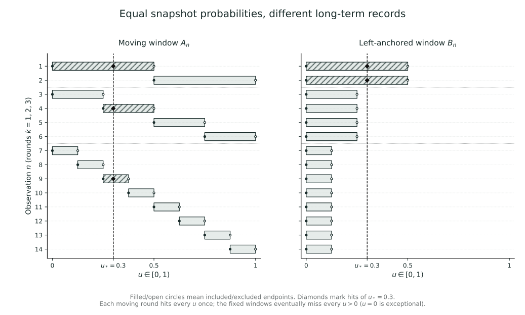
Equally small hit probabilities, different individual records In round k the moving window is [j/2^k,(j+1)/2^k), with j from 0 to 2^k−1. Each hit probability is 2^−k. The windows partition [0,1) each round: every fixed point is hit exactly once and has value 0 at the other windows, so the moving sequence has no pointwise limit. The left-end window [0,2^−k) eventually misses each u>0; u=0 is a null-probability exception. The static frames explain the partition mechanism. The deterministic controls aid observation, not the proof of an infinite conclusion.
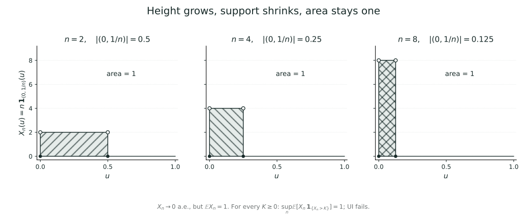
Height carries away the disappearing width X_n=n·1_(0,1/n), with both endpoints excluded; endpoints do not affect area. Every fixed u>0 eventually leaves the spike, and the value at u=0 is always 0, yet the integral remains 1. For any K≥0 choose n>K: the expectation beyond the threshold is still 1. Thus sup_n E[X_n·1_{X_n>K}]=1 and uniform integrability fails. Common scales and equal-area hatching distinguish shrinking probability from persistent average contribution.
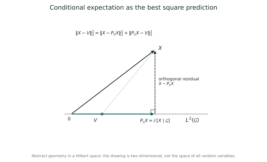
What prediction retains, and where the residual points Write P_G X=E[X|G]. This is an abstract two-dimensional sketch of L² geometry, not a claim that all random variables live in two dimensions. The residual X−P_G X is orthogonal to all of L²(G). For any other observable predictor V, E[(X−V)²] equals E[(X−P_G X)²]+E[(P_G X−V)²]. This orthogonal mechanism explains best squared prediction; the diagram does not replace the existence and uniqueness proof.
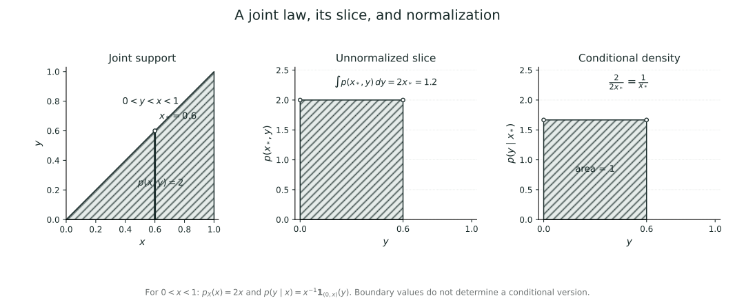
From a triangular region to a normalized vertical slice Left: the support of joint density 2. Middle: at x*=0.6 the slice still has density 2 along y, whose integral is the marginal density m(x*)=2x*=1.2. Right: division by 2x* gives height 1/x* on (0,x*) and area 1. Slice mass here is a marginal density, not P(X=x*): the singleton still has probability zero. Disintegration identifies the density kernel. At x=0 choose a separate version; do not use the 1/x formula.
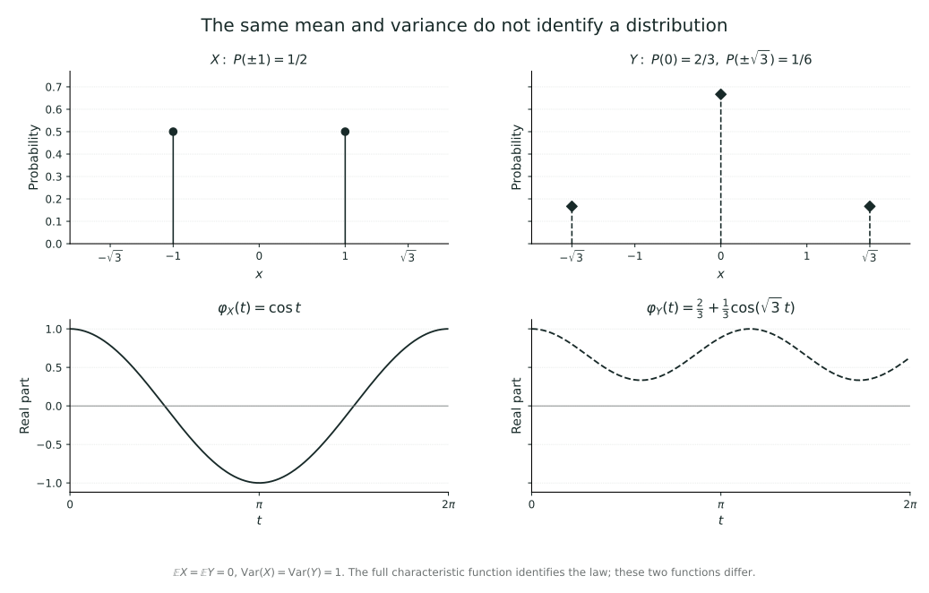
Equal means and variances, different frequency readings X takes ±1 with probability 1/2 each. Y has mass 2/3 at 0 and mass 1/6 at each of ±√3. Both have mean 0 and variance 1, but φ_X(t)=cos t and φ_Y(t)=2/3+(1/3)cos(√3t) differ. Symmetry makes both imaginary parts zero. Low-order moments record only limited local information near the origin; the complete characteristic function identifies the whole law. A finite plot is illustrative; uniqueness uses every real frequency.
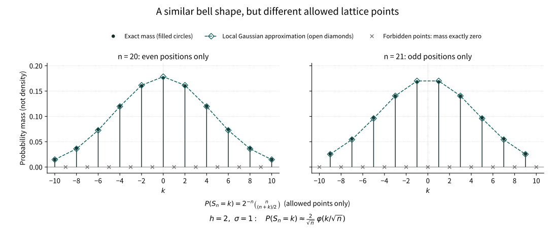
Similar bell-shaped profiles, different allowed parity classes Independent steps take ±1 with probability 1/2 each; n=20 on the left, n=21 on the right. Filled circles and stems are exact masses; dashed open diamonds show (2/√n)φ(k/√n) at allowed sites, not the continuous density itself. Maximal span h=2 explains the factor 2; the other parity class has mass exactly zero. Only |k|≤10 is plotted; the shared source retains the full support and exact values. No simulation is used. The plot gives no convergence rate and does not replace the local-CLT proof; total variation requires the next section’s discretized Gaussian.
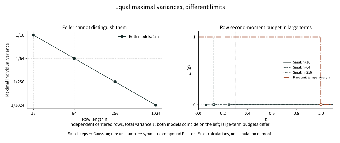
The same Feller bound, entirely different large-term budgets Each row has n terms and total variance 1. Small terms take ±1/√n equally; rare terms take ±1 with probability 1/(2n) each and 0 otherwise. Both maximal variances are 1/n, so both satisfy Feller. For fixed 0<ε<1, however, the small-step L_n(ε) is eventually 0 while the rare-jump budget stays 1. The vertical dotted line marks a fixed ε=0.3. Curves are exact second-moment calculations without simulation; a finite plot does not replace the CLT proof below.