Haobai Wang · Public reading edition · ch07-en-a253bca6b555
This content fingerprint identifies the text, not academic final approval or an independent proof of authorship.
SHA-256: a253bca6b555aafd23b0d0e86a532bd192cc6183ae7896087bd3613bf3f71940
The Mathematics of Chance
Volume II · Probability in an Infinite World
Chapter 7: What Does Convergence Mean? Four Limits in a Random World
At the end of Chapter 6, we left a spike that was growing narrower and taller.
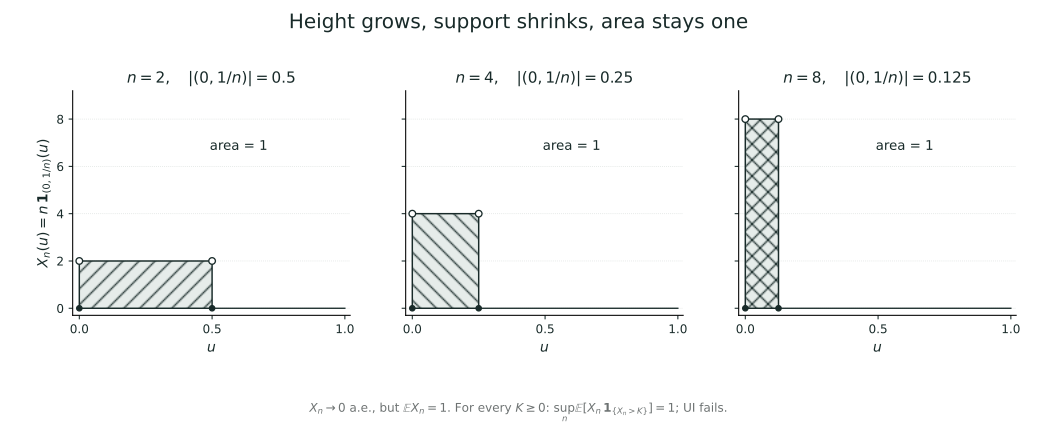
Choose a point U uniformly from the interval [0,1], and set
X_n=n\mathbf1_{\{0<U<1/n\}}.For every fixed sample point, the spike eventually leaves it behind. Thus X_n\to0 holds almost surely. Yet however large we make n,
\mathbb E[X_n]=1.We have witnessed one limit without obtaining another.
Is the integral refusing to cooperate, or has our understanding of ‘getting closer’ been missing something all along?
Now turn the question around. Suppose the probability of an exception at observation n tends to zero. Can we guarantee that an actual record of observations eventually contains no more exceptions?
Once again, the answer can be no.
The spike reminds us that stability along individual records need not control average loss. Our next example will remind us that something rare at any particular moment may nevertheless recur throughout a lifetime.
To understand these two failures, we must return to a word we have used repeatedly since Chapter 2: convergence.
7.1 A Shrinking Window That Keeps Passing Everyone
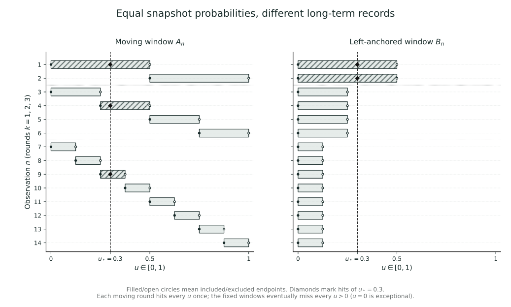
Use Lebesgue probability once more on \Omega=[0,1). Think of this interval as the collection of all possible observation records; selecting a particular u selects one record.
In the first round, divide the interval in half and open the two windows in turn:
[0,1/2),\qquad[1/2,1).In the second round, divide it into four pieces and again open the windows from left to right:
[0,1/4),\quad[1/4,1/2),\quad[1/2,3/4),\quad[3/4,1).Round k contains 2^k windows, each of width 2^{-k}. Only records lying in the current window register an exception at that observation.
This picture can be made precise. Write
N_0=0,\qquad N_k=\sum_{r=1}^k2^r=2^{k+1}-2,and, for k\ge1 and 0\le j<2^k, define
A_{N_{k-1}+j+1}
=\left[\frac j{2^k},\frac{j+1}{2^k}\right),
\qquad Y_n=\mathbf1_{A_n}.
As the observation number n increases, its round number k increases too, so
P(Y_n=1)=P(A_n)=2^{-k}\longrightarrow0.But every fixed u\in[0,1) lies in exactly one window in every round. Every record therefore contains infinitely many exceptions.
Each round also contains at least one other window that misses it. Hence, for every u,
\limsup_{n\to\infty}Y_n(u)=1,
\qquad
\liminf_{n\to\infty}Y_n(u)=0.
The sequence does not even have a pointwise limit.
Often called the ‘typewriter sequence’, this example sweeps across the interval like a cursor. Its windows shrink, but they never stop seeking new sample points. Fewer people see an exception at each observation, yet nobody is promised that it will eventually stop being their turn.
Now keep windows of the same sizes fixed at the left endpoint. If n belongs to round k, set
B_n=[0,2^{-k}),\qquad Z_n=\mathbf1_{B_n}.We still have
P(Z_n=1)=P(Y_n=1).But for every u>0, all windows lie to its left from some round onward. Thus Z_n(u)\to0; only zero is exceptional, and zero has probability zero.
The two sequences have exactly the same distribution at each observation. One tends to zero almost surely; the other keeps oscillating along every record.
We encountered something similar in Chapter 1. Fairness in each of two games did not determine their joint outcome. Now the exception probability at each time likewise fails to determine the fate of an infinite record.
What is missing, once again, is the connection between different observations.
7.2 From the Digits of One Real Number to Infinitely Many Events
Using an entire interval as a random experiment is not merely a way to manufacture counterexamples.
Borel’s 1909 paper Les probabilités dénombrables et leurs applications arithmétiques connected countable probability with arithmetic questions. Along this line of inquiry, the infinite digit expansion of a real number becomes a natural entry into infinite random records. Original publication record
We reconstruct the question below in the modern language of Lebesgue probability. Neither the modern notation nor the proof that follows is presented as Borel’s original wording.
Choose U uniformly in [0,1), and write its binary expansion:
U=0.\xi_1\xi_2\xi_3\cdots\quad\text{(binary)}.For dyadic rationals with two expansions, consistently choose the one that is eventually zero. These points form a countable set and do not affect the probability conclusions below.
Specifying the first m digits, for example 0101\cdots, places the number in a half-open interval of length 2^{-m}. Thus every specified digit string of length m has probability 2^{-m}.
To specify any finite set of digit positions, go as far as the largest position and count the unspecified digits. This gives
P(\xi_{i_1}=a_1,\ldots,\xi_{i_r}=a_r)=2^{-r},
\qquad a_j\in\{0,1\}.
These digits are therefore independent, fair Bernoulli random variables.
Pause over what has happened: we did not begin by assuming an infinite coin-tossing space that had yet to be constructed. The length measure of Chapter 5 has already accommodated an entire sequence of independent tosses inside one random real number.
We can now ask whether the digit 1 eventually accounts for half of an infinite expansion. We can also ask whether certain increasingly rare digit patterns nevertheless keep appearing.
The first question leads toward the strong law of large numbers. The second first requires us to identify precisely the event called ‘keeps appearing’.
For a sequence of measurable events A_1,A_2,\ldots, at least one occurrence from observation N onward corresponds to
E_N=\bigcup_{n\ge N}A_n.No matter how far we move the starting point N, there is another occurrence afterward. This corresponds to
\limsup_{n\to\infty}A_n
=\bigcap_{N=1}^{\infty}\bigcup_{n\ge N}A_n.
This is the event that A_n occur infinitely often, usually abbreviated as \{A_n\ \mathrm{i.o.}\}. Here i.o. stands for infinitely often.
It does not mean ‘occurs at some exceptionally distant time’. It tests all arbitrarily distant starting points at once.
We can assign a probability to this statement about infinite time because Chapter 5 permits countable unions and intersections. Abstract foundations have become the grammar needed to describe an infinite record.
7.3 How Can All Distant Exceptions Disappear Together?
If all we know is P(A_n)\to0, the moving windows of the first section have already shown that the matter is not simple.
But what if the sum of the probabilities of all distant exceptions is itself small?
Countable subadditivity immediately gives
P(E_N)\le\sum_{n\ge N}P(A_n).Consequently, whenever
\sum_{n=1}^{\infty}P(A_n)<\infty,the tail sum on the right tends to zero. Moreover, E_N decreases as N increases, and P(E_1)\le1. Continuity from above therefore gives
P(A_n\ \mathrm{i.o.})
=\lim_{N\to\infty}P(E_N)=0.
This is the first direction of the Borel–Cantelli lemma: if the exception probabilities are summable, almost every record contains only finitely many exceptions.
The proof is short, but it changes the level of the question. A probability at one time has been replaced by an upper bound covering all future times. ‘Becoming rarer’ has thereby become ‘eventually stopping’.
No independence was used. The exceptions may depend on one another in any way; a finite total probability budget prevents them from continuing infinitely often on a set of records of positive probability.
We can see the same fact again through the integration language of Chapter 6. Let
N(\omega)=\sum_{n=1}^{\infty}\mathbf1_{A_n}(\omega)count the total number of exceptions, allowing infinity. By monotone convergence,
\mathbb E[N]=\sum_nP(A_n)<\infty.A nonnegative random variable with finite expectation cannot equal infinity with positive probability: for every M>0, P(N\ge M)\le\mathbb E[N]/M, and then let M\to\infty.
For a second time, we obtain N<\infty almost surely.
The same fact has two faces. In terms of events, the probabilities of tail unions vanish; in terms of integration, a finite average count rules out an infinite count. Measure and integration meet here in the study of infinite random records.
Do not reverse the statement, however. \mathbb E[N]=\infty does not guarantee N=\infty. Chapter 6 already showed that a random variable finite almost surely can have infinite expectation.
When the sum of probabilities diverges, we therefore need another condition.
7.4 How Does Independence Bring Rare Events Back Again?
Suppose A_n are mutually independent and \sum_nP(A_n)=\infty.
The probability of no occurrence between observations N and M is
P\left(\bigcap_{n=N}^MA_n^c\right)
=\prod_{n=N}^M(1-P(A_n))
\le\exp\left(-\sum_{n=N}^MP(A_n)\right).
The last step uses only 1-x\le e^{-x}. Fix N and let M\to\infty. The right side tends to zero; by continuity from above, the left side tends to P(\bigcap_{n\ge N}A_n^c).
Thus, from any given starting point, the probability of never seeing another occurrence is zero. Finally take the union over the countably many starting points to obtain
\boxed{
\sum_nP(A_n)=\infty,\quad A_n\text{ are mutually independent}
\quad\Longrightarrow\quad
P(A_n\ \mathrm{i.o.})=1.
}
This is the second direction. Independence turns ‘each opportunity can be missed’ into ‘infinitely many factors exhaust the chance of missing every opportunity forever’.
Independence is not the weakest possible sufficient condition, but it already makes the mechanism clear. We cannot merely replace a convergent probability sum by a divergent one and reverse the preceding lemma’s conclusion.
For example, on (0,1) take A_n=(0,1/n). The probability sum is the divergent harmonic series, yet every fixed u>0 eventually leaves all the A_n. The probability of infinitely many occurrences is still zero.
These events keep shrinking into the same region. They do not offer most records any new opportunities.
For an independent example whose probabilities tend to zero while occurrences continue infinitely often, we need not invoke an infinite product measure theorem in advance. Use the independent binary digits from the second section and divide them successively into disjoint finite blocks. In round k, use 2^k blocks of length k, each using digit positions never used before. Let one event be that every digit in a block is 1.
The events for different blocks are mutually independent. Each event in round k has probability 2^{-k}, and the sum of all probabilities in that round is
2^k\cdot2^{-k}=1.Numbering the rounds in order, the individual probabilities tend to zero, but their sum diverges. The second lemma therefore says that these events occur infinitely often in the digit record of almost every random real number.
Becoming rarer does not mean becoming less likely to meet again. The size of one opportunity and the way opportunities accumulate throughout a lifetime are different information.
Cantelli studied the limiting relationship between probability and frequency in his 1917 paper Sulla probabilità come limite della frequenza; his 1935 Considérations sur la convergence dans le Calcul des probabilités addressed convergence in probability theory directly. These original documents remind us that today’s neatly arranged language of convergence grew from a long effort to distinguish different limiting requirements, rather than from casually giving several names to one idea. 1917 academy catalogue; 1935 original text
In the historical discussion of his 1935 lectures, Cantelli returned specifically to a distinction easily hidden by the language of frequencies: a frequency being close to the true probability with high probability at one late time is a different promise from all frequencies being close simultaneously from some time onward. This is precisely the difficulty we have faced on our way here from Chapter 2. Infinitely many times cannot be covered merely by a guarantee for one large sample. Part III of the original text
This chapter uses modern statements and proofs of Borel–Cantelli. It does not assert that the historical papers used exactly our terminology and assumptions.
7.5 The Coin of Chapter 2 Finally Receives an Answer for Individual Records
We can now return to empirical frequencies.
For independent fair coins, Chapter 2 proved that the probability of a fixed deviation from 1/2 tends to zero. Using the variance alone gives the estimate
P\left(\left|\frac{S_n}{n}-\frac12\right|>\varepsilon\right)
\le\frac1{4n\varepsilon^2}.
Although the right side tends to zero, it is not summable. This bound does not entitle us to announce that exceptions occur only finitely often.
That does not make the stronger conclusion false. It only means that this estimate is not sharp enough.
Set \eta_i=\xi_i-1/2. Then the \eta_i are independent, take values \pm1/2, and have mean zero. In the fourth-power expansion, every term containing an odd power of some variable has expectation zero. Only terms with one index appearing four times, or two distinct indices appearing twice each, remain:
\begin{aligned}
\mathbb E\left(\sum_{i=1}^n\eta_i\right)^4
&=\sum_i\mathbb E\eta_i^4
+6\sum_{i<j}\mathbb E\eta_i^2\mathbb E\eta_j^2\\
&=\frac n{16}+\frac{6}{16}\binom n2
=\frac{3n^2-2n}{16}.
\end{aligned}
Consequently, Markov’s inequality for nonnegative variables gives
P\left(\left|\frac{S_n}{n}-\frac12\right|>\varepsilon\right)
\le\frac{3}{16\varepsilon^4n^2}.
This time the probability bound is summable. For each fixed \varepsilon>0, the first Borel–Cantelli lemma says that this error is exceeded only finitely often, almost surely.
To obtain convergence, however, we cannot keep just one error threshold fixed. Apply the conclusion separately to \varepsilon=1,1/2,1/3,\ldots, then intersect these countably many probability-one events. On one common probability-one set, for each m we eventually have
\left|\frac{S_n}{n}-\frac12\right|\le\frac1m.Only now have we truly shown that
\boxed{\frac{S_n}{n}\longrightarrow\frac12\quad\text{almost surely}.}We did not require independence between deviation events at different sample sizes; in fact, they are usually highly dependent. Independence of the original coin increments was used only in calculating the fourth moment.
This distinction matters. We must follow the proof to see where independence enters, rather than use the word as a vague incantation.
The same calculation works for independent, identically distributed, bounded Bernoulli variables of mean p. If \eta_i=\xi_i-p, then |\eta_i|\le1, and the expansion gives \mathbb E(\sum_i\eta_i)^4\le3n^2. This already supplies a summable bound of the same kind. Thus, for any fixed p\in[0,1], Bernoulli frequencies converge almost surely to p.
This is a complete proof of a strong law of large numbers, but it uses bounded increments. The strong law for general integrable i.i.d. variables requires further tools, including truncation; this fourth-moment calculation cannot replace that argument.
7.5.1 From One Digit to Every Finite Pattern of a Real Number
We can take the digit-expansion question a step further.
In any integer base b\ge2, intervals of length b^{-m} show that the digits of a uniform real number are independent and uniform on \{0,\ldots,b-1\}. Fix a digit string w of length r. Its probability of appearing from a given position is b^{-r}.
Occurrences starting at adjacent positions overlap, so they cannot simply be treated as independent coin tosses. Group the starting positions into r residue classes modulo r. Within each group the digit blocks do not overlap, so their indicator variables are i.i.d.
The bounded Bernoulli strong law applies to each group. Its occurrence frequency tends to b^{-r}, while the proportions of the groups among starting positions up to n tend to 1/r. Recombining the groups, the frequency over all starting positions therefore also tends to b^{-r}.
For fixed b,r,w, this happens on a probability-one set. There are only countably many choices of integer base, string length and finite digit string. Taking another countable intersection, we obtain: almost every real number has every finite digit string occurring with its expected frequency in every integer base.
This gives a modern route to the probabilistic conclusion of absolute normality. We have proved an almost-everywhere property, not thereby established the property for a particular specified real number, such as \sqrt2.
From the variance of a single coin, to stable frequencies along a record, to the digit structure of almost all real numbers, we have not changed the concept of probability. We have changed how we observe an infinite experiment.
7.6 Two Meanings of ‘Eventually’: Fix a Record First, or Fix a Time First?
Only now is it time to give formal names to the two requirements.
In what follows, we first study real-valued measurable random variables X_n,X on one probability space (\Omega,\mathcal F,P). When we reach convergence in distribution, we will explain explicitly why the variables no longer need to share that space.
Almost sure convergence means that there is a measurable null set N such that X_n(\omega)\to X(\omega) in the usual real-number sense for every \omega\notin N. We write
X_n\xrightarrow{\mathrm{a.s.}}X.It fixes a record first and then follows that record indefinitely. Different records may require entirely different waiting times; almost sure convergence supplies no common deadline that works for everyone.
Convergence in probability, by contrast, requires that for every \varepsilon>0,
P(|X_n-X|>\varepsilon)\longrightarrow0,
\qquad\text{written }X_n\xrightarrow P X.
At each fixed late time, it measures the probability of the records still failing to be close enough. The membership of that group may keep changing.
The moving windows of the first section satisfy Y_n\xrightarrow P0 but have no almost sure limit; the left-anchored windows Z_n tend to zero almost surely. Since the two sequences have identical distributions at each time, their difference must lie in the joint structure across time.
7.6.1 Why Does Stability Along Records Make the Fraction of Exceptions Vanish?
Suppose X_n\to X almost surely. Fix \varepsilon>0 and set
E_N(\varepsilon)=\bigcup_{n\ge N}\{|X_n-X|>\varepsilon\}.Almost every record eventually stops exceeding this error, so \bigcap_NE_N(\varepsilon) is a null event. Since E_N decreases and the probability is finite, P(E_N)\to0. Moreover,
P(|X_N-X|>\varepsilon)\le P(E_N(\varepsilon))\to0.We have obtained
X_n\xrightarrow{\mathrm{a.s.}}X\quad\Longrightarrow\quad X_n\xrightarrow P X.From Chapter 6’s perspective, we could instead apply dominated convergence to the bounded indicator functions \mathbf1_{\{|X_n-X|>\varepsilon\}}. Both proofs rely on the same fact: the entire probability space has finite total mass.
For a general infinite measure, the implication cannot be carried over unchanged. On the real line, \mathbf1_{(n,n+1)} tends pointwise to zero, yet the set where it exceeds 1/2 always has measure 1. Mass can keep moving toward infinity. The finite total mass of a probability space rules out this form of escape.
7.6.2 The Order of Quantifiers Is a Mathematical Structure Too
For fixed \varepsilon>0, convergence in probability says
\lim_{n\to\infty}P(|X_n-X|>\varepsilon)=0.Almost sure convergence requires, for each such threshold, that combining the exceptions at all distant times still leaves a probability that vanishes:
\lim_{N\to\infty}P\left(\bigcup_{n\ge N}\{|X_n-X|>\varepsilon\}\right)=0.Checking the second formula for the countably many thresholds \varepsilon=1/m is equivalent to almost sure convergence. It coordinates future times in a way the first formula does not.
We can turn this coordination into a stronger geometric picture. Given \delta>0, choose N_m for each m so that
P(E_{N_m}(1/m))<\delta2^{-m}.Remove H=\bigcup_mE_{N_m}(1/m); then P(H)<\delta. On H^c, for every m and all n\ge N_m, we have |X_n-X|\le1/m. Convergence is therefore uniform on H^c.
This proves the Egorov phenomenon on a finite measure space: almost-everywhere convergence becomes uniform after discarding an arbitrarily small probability set. It does not give one fixed null set outside which convergence is uniform on the entire remaining space. ‘Arbitrarily small’ cannot simply be replaced by ‘zero’.
Almost sure convergence and convergence in probability differ not because one sounds more like everyday language, but because they arrange the quantifiers over time and samples in different orders.
7.7 If the Whole Sequence Will Not Settle Down, Can We Choose a Sparser Timeline?
The moving window forces us to admit that convergence in probability cannot simply be upgraded to almost sure convergence.
But not every hope for individual records is lost. Convergence in probability lets us wait long enough to make the probability of a specified error arbitrarily small. Why not organize those waits?
Suppose X_n\xrightarrow P X. First choose n_1 so that P(|X_{n_1}-X|>1/2)<1/2; then choose a larger n_2 so that the probability of an error exceeding 1/4 is less than 1/4. Continuing recursively, we obtain strictly increasing n_j satisfying
P(|X_{n_j}-X|>2^{-j})\le2^{-j}.Now the exception probabilities are summable. Borel–Cantelli says that, along almost every record, only finitely many j violate |X_{n_j}-X|\le2^{-j}. Hence
\boxed{X_{n_j}\xrightarrow{\mathrm{a.s.}}X.}The selected timeline does not depend on the sample point. We first choose n_j using the probabilities of the entire collection of records, and then the same timeline works for almost all records.
This is quite different from selecting a good subsequence separately for each record. That selection could depend on the record and would not give the common probability conclusion obtained here.
Moreover, every subsequence of the original sequence still converges in probability, so each admits a further subsequence converging almost surely. We obtain an exact criterion:
Real-valued random variables X_n converge in probability to X if and only if every subsequence has a further subsequence converging almost surely to X.
We have proved the forward direction. The reverse direction deserves a complete look as well.
If convergence in probability fails, there are \varepsilon,\delta>0 and a subsequence n_k such that, for every k,
P(|X_{n_k}-X|>\varepsilon)\ge\delta.By assumption, this subsequence has a further subsequence tending almost surely to X. But almost sure convergence has already been shown to imply convergence in probability, so the same deviation probabilities must tend to zero, contradicting their lower bound \delta.
Notice the word ‘every’ in the criterion. The existence of just one good subsequence is far from enough. For example, the deterministic sequence 0,1,0,1,\ldots has an identically zero subsequence but does not converge to zero in probability.
This is an idea we will use repeatedly: rather than force the entire sequence to have a pointwise property, require that after every extraction there remains a chance to extract again and recover that property.
7.7.1 Why Cannot One Limit Be Two Different Random Variables?
If X_n\xrightarrow P X and X_n\xrightarrow P Y, the triangle inequality gives, for every \varepsilon>0,
P(|X-Y|>\varepsilon)
\le P(|X-X_n|>\varepsilon/2)
+P(|X_n-Y|>\varepsilon/2).
Letting n\to\infty makes the left side zero. Taking a countable union over thresholds 1/m then gives X=Y almost surely.
The limit is therefore unique, but only up to a null set. This agrees with the integration language of Chapter 6: probabilities and integrals cannot distinguish variables that differ only on a measurable null set. Such resolution is not a gap in the theory; it is the scale of information the theory chose from the outset.
7.8 If Errors Are Rare, Why Can Average Loss Remain Large?
Return to the spike X_n=n\mathbf1_{\{0<U<1/n\}} from Chapter 6. It tends to zero almost surely, hence also in probability. But each rare hit produces an increasingly large value, leaving the average loss constantly equal to 1.
Counting only whether an error exceeds a threshold discards how serious it becomes afterward.
We can make that statement precise. For D_n=|X_n-X|, first cap the loss at 1. If 0<\varepsilon<1, then
\varepsilon P(D_n>\varepsilon)
\le\mathbb E[\min(1,D_n)]
\le\varepsilon+P(D_n>\varepsilon).
The left inequality integrates over the exception set. The right follows by dividing the space into D_n\le\varepsilon and its complement.
Convergence in probability is therefore equivalent to
\mathbb E[\min(1,|X_n-X|)]\longrightarrow0.So convergence in probability can also be described through average loss. But this loss has a ceiling: an error of 10 and an error of a million become indistinguishable after they reach it.
If we remove the cap and genuinely care about the average magnitude of the error, the natural requirement becomes
\mathbb E|X_n-X|\longrightarrow0.This is called L^1 convergence.
To penalize large errors more heavily, we can consider the pth power. For 1\le p<\infty, assuming finite absolute moments of order p, we write
\|Z\|_p=(\mathbb E|Z|^p)^{1/p},
\qquad
X_n\xrightarrow{L^p}X
\quad\Longleftrightarrow\quad
\mathbb E|X_n-X|^p\longrightarrow0.
Here the space L^p consists of random variables with finite moments of order p, identifying variables equal almost everywhere. The quantity \|\cdot\|_p is its usual norm. Further structure, such as completeness, is not a prerequisite for the arguments below; first we ask why this quantity measures random error appropriately.
For p=2, we ask that mean square error vanish. This connects directly with Chapter 2’s variance bounds: for an unbiased estimator, mean square error equals variance. For p=1, we require the average absolute error to vanish, without letting positive and negative errors cancel.
7.8.1 Why Does Average Error Control Exception Probabilities?
On \{|X_n-X|>\varepsilon\}, we have |X_n-X|^p>\varepsilon^p, so
P(|X_n-X|>\varepsilon)
\le\frac{\mathbb E|X_n-X|^p}{\varepsilon^p}.
Thus L^p convergence necessarily implies convergence in probability.
It still does not guarantee convergence along the entire sequence of individual records. The moving window offers a particularly vivid counterexample: for any fixed finite p\ge1,
\mathbb E|Y_n|^p=P(A_n)\to0,Hence Y_n\to0 in every such L^p sense, although not a single record tends to zero.
Penalizing the height of an error and arranging the times at which errors occur are still different tasks.
Conversely, the spike disappears along every record without disappearing in L^1. Consequently, L^p and almost sure convergence cannot simply be arranged on one line from weak to strong.
7.8.2 How Are Different Average Losses Related?
On a probability space, if 1\le q\le p<\infty, then
\|Z\|_q\le\|Z\|_p.The estimate needed here can be proved without assuming the full Hölder theory. Let a=\mathbb E|Z|^p. If a=0, the result is immediate. If 0<a<\infty, take r=q/p\le1 and use the tangent-line inequality t^r\le rt+1-r for nonnegative numbers to obtain
\mathbb E\left(\frac{|Z|^p}{a}\right)^r
\le r\mathbb E\frac{|Z|^p}{a}+1-r=1.
Rearrangement gives the desired conclusion. Thus L^p convergence implies L^q convergence.
The reverse direction generally fails. For q<p, take
H_n=n^{1/p}\mathbf1_{\{0<U<1/n\}},Then
\mathbb E|H_n|^q=n^{q/p-1}\to0,
\qquad \mathbb E|H_n|^p=1.
A large error becomes cheap under a lower power while leaving a non-negligible contribution under a higher power.
Defining L^\infty error through the essential supremum imposes a stronger requirement. Even though \mathbf1_{\{0<U<1/n\}} almost surely and in every finite L^p, its essential supremum stays equal to 1. For 0<p<1 one can also study \mathbb E|X_n-X|^p\to0, but the corresponding (\mathbb E|Z|^p)^{1/p} is no longer a norm. Our main discussion uses p\ge1.
7.8.3 What Does Dominated Convergence Now Explain?
If X_n\to X almost surely, with |X_n|\le G and \mathbb E G^p<\infty, then |X|\le G holds on the same probability-one set. Consequently,
|X_n-X|^p\le2^{p-1}(|X_n|^p+|X|^p)\le2^pG^p.The dominated convergence theorem of Chapter 6 immediately yields L^p convergence.
This theorem does not declare two convergence notions equivalent. It adds a common constraint across all times: no increasingly tall spike can evade the same integrable dominating function.
If we do not want to demand a common upper bound, can we find a condition that is exactly sufficient? This question will soon lead us to uniform integrability.
Before pursuing average loss, however, we should identify an earlier kind of limit. Exactly what form of approximation did Chapter 3’s bell curve describe?
7.9 Which Random Variable Is the Bell Curve Approaching?
Chapter 3 wrote
\frac{S_n-n\mu}{\sigma\sqrt n}\xrightarrow d N(0,1).The right side first specifies a distribution, not some record already present among the original coin tosses.
We can define S_n for every sample size on the same space. But the central limit theorem does not thereby specify a particular Z and guarantee that the standardized error along every record gets closer to that Z.
An example requiring no asymptotic calculation brings this difference into view.
On a space with just two equally likely outcomes, take P(X=0)=P(X=1)=1/2 and set
X_{2n}=X,\qquad X_{2n-1}=1-X.Each X_n has the same distribution as X. Their histograms have been identical from the very first day.
Yet along every record the values keep alternating between 0 and 1. In particular,
P(|X_{2n-1}-X|>1/2)=1.There is therefore no convergence in probability to this X.
If we retain only the individual probability distributions, all this alternation becomes invisible. Convergence in distribution studies limits precisely at that level.
For real-valued random variables, let
F_n(x)=P(X_n\le x),\qquad F(x)=P(X\le x).We define X_n\xrightarrow d X to mean that F_n(x)\to F(x) at every continuity point x of F. Another common notation is X_n\Rightarrow X.
The X_n may perfectly well live on different spaces (\Omega_n,\mathcal F_n,P_n): replace F_n by P_n(X_n\le x). The limiting variable may live on yet another space. We compare only distributions on the real line.
Why not require convergence at every point? Consider deterministic variables X_n=1/n and X=0. Their values approach zero at every sample point, but
F_n(0)=0,\qquad F(0)=1.The problem is not the approximation of values. An atom suddenly appears at the boundary of the interval ( -\infty,0]. Such a boundary choice should not destroy a limit that ought to hold.
The continuity-point restriction therefore distinguishes closeness of distributions from the assignment of mass at a sharp boundary.
7.9.1 Why Does Convergence in Probability Bring Distributions Closer?
If X_n\xrightarrow P X, then on the event \{|X_n-X|\le\varepsilon\},
X\le x-\varepsilon\Longrightarrow X_n\le x,
\qquad
X_n\le x\Longrightarrow X\le x+\varepsilon.
and hence
F(x-\varepsilon)-P(|X_n-X|>\varepsilon)
\le F_n(x)
\le F(x+\varepsilon)+P(|X_n-X|>\varepsilon).
First let n\to\infty, then \varepsilon\downarrow0. If x is a continuity point of F, both endpoints tend to F(x), giving F_n(x)\to F(x).
This proves that convergence in probability implies convergence in distribution. The alternating Bernoulli example has already disproved the reverse direction.
An important exception occurs when the limit is a constant c. If X_n\xrightarrow d c, then for every \varepsilon>0 the points c-\varepsilon and c+\varepsilon are continuity points of the limiting distribution function, so
P(|X_n-c|>\varepsilon)
\le F_n(c-\varepsilon)+1-F_n(c+\varepsilon)\to0.
Thus convergence in distribution to a constant is equivalent to convergence in probability to that constant.
This explains a familiar experience. The weak law of large numbers has a constant limit, so concentration at the distributional level suffices. The central limit theorem has a genuinely random limit, so distributional convergence cannot simply be promoted to closeness of values in the original space.
7.10 Beyond Interval Endpoints: Stabilizing Every Continuous Observation
Distribution functions provide convenient coordinates on the real line, but do not look like a definition suited to random functions or random trees. What should play the role of ‘X\le x’ for a path?
First change our viewpoint on the real line itself.
Suppose an instrument reports a bounded continuous function f(X) instead of the truth or falsity of a sharp event. Compare its average readings under two distributions. A natural requirement is
\mathbb E[f(X_n)]\longrightarrow\mathbb E[f(X)]
\quad\text{for every bounded continuous }f:\mathbb R\to\mathbb R.
This is exactly equivalent to the distribution-function definition. We prove it so that we can be sure the new viewpoint has not lost the original limit.
7.10.1 How Can a Continuous Instrument Approximate an Interval?
First suppose expectations of all bounded continuous readings converge. Given x and \delta>0, construct two continuous ramps. One stays at 1 before x-\delta and decreases to 0 at x; the other stays at 1 before x and decreases to 0 at x+\delta. Elsewhere they remain at 0 or 1.
Call them \ell_\delta,u_\delta. Then
\ell_\delta(t)\le\mathbf1_{\{t\le x\}}\le u_\delta(t).Take expectations under X_n and pass to limits to obtain
F(x-\delta)\le\liminf_nF_n(x)
\le\limsup_nF_n(x)\le F(x+\delta).
If F is continuous at x, letting \delta\downarrow0 gives the desired distribution-function convergence.
The ramps approach the boundary gradually rather than leaping across it. When the limiting distribution gives that boundary no mass, the gradual approach leaves no error.
7.10.2 How Do Interval Probabilities Control Every Continuous Reading?
Conversely, we know only interval probabilities but want to recover arbitrary continuous readings across the entire real line. The difficulty has two layers: the reading changes with position, and the line has no end. First keep almost all probability in a bounded interval, then approximate readings there using finitely many graduations. Only then can the distribution function’s information take charge of each graduation.
Suppose F_n tends to F at every continuity point of F, and take bounded continuous f with |f|\le M. If M=0, there is nothing to prove.
First choose continuity points a<b sufficiently far apart that
F(a)+1-F(b)<\eta.This is possible because a distribution function tends to 0 and 1 at the two ends of the line and has at most countably many discontinuities. The latter fact has a simple explanation: there are at most m jumps of size at least 1/m, and all positive jumps form a countable union of these finite sets.
Convergence at the endpoints ensures that, for large enough n, P(X_n\notin(a,b])<2\eta; the corresponding tail probability for the limit is less than \eta. The total error in the two tail readings is thus at most 3M\eta.
Boundedness has controlled the distant readings. What remains is variation nearby. On the compact interval [a,b], f is uniformly continuous: one sufficiently fine system of graduations works at every position. Divide the interval into finitely many sufficiently short pieces (t_{j-1},t_j], with all endpoints continuity points of F, so that the oscillation of f on each piece is less than \eta. Choose one representative c_j per piece.
The integral over the interior can then be approximated by a finite sum:
\sum_j f(c_j)\,[F_n(t_j)-F_n(t_{j-1})].Each coefficient converges to the corresponding limiting interval probability, and each of the two approximation errors is at most \eta. Hence
\limsup_n|\mathbb Ef(X_n)-\mathbb Ef(X)|
\le 2\eta+3M\eta.
Let \eta\downarrow0 to finish the proof.
Looking back, the two approximations had different responsibilities: control probability far away, then oscillation nearby. Finite partitions on the real line connect the two tasks and leave a clue for our later passage to general spaces.
‘Bounded’ and ‘continuous’ each do a particular job. Boundedness prevents rare large values from dominating the reading; continuity prevents infinitesimal movements from crossing a sharp boundary carrying mass.
Remove the first, and Chapter 6’s spike makes the expectation of f(x)=x misbehave. Remove the second: for X_n=1/n\to0, the readings of f=\mathbf1_{\{0\}} remain zero, but the limiting reading is 1.
These restrictions are not arbitrary concessions to the proof. They correspond exactly to two different ways a limit can fail.
The four limits have now separated: individual records, exception probabilities, average losses and continuous readings of distributions. Yet the spike’s original question remains. Is there a more flexible condition than one common integrable bound that makes average loss obey a limit?
7.11 What the Spike Carries Away Is Average Loss, Not Probability
Look once more at X_n=n\mathbf1_{\{0<U<1/n\}}. Its probability of being nonzero is only 1/n, but whenever n>K,
\mathbb E\bigl[|X_n|\mathbf1_{\{|X_n|>K\}}\bigr]=1.However high we place the ‘large value’ threshold K, a taller spike puts the entire average loss beyond it.
The issue is therefore not merely \sup_n\mathbb E|X_n|<\infty. We also need this finite average loss not to reconcentrate in regions of larger and larger values.
A family \mathcal X of integrable random variables is called uniformly integrable if
\boxed{
\lim_{K\to\infty}\sup_{Y\in\mathcal X}
\mathbb E\bigl[|Y|\mathbf1_{\{|Y|>K\}}\bigr]=0.
}
Uniform integrability is commonly abbreviated UI. When \mathcal X=\{X_n:n\ge1\}, we say the sequence is uniformly integrable.
Every individual integrable variable has tail expectations tending to zero. Dominated convergence gives this immediately: |Y|\mathbf1_{\{|Y|>K\}}\to0, dominated by the integrable |Y|.
The new requirement is that one K work simultaneously for the entire family. Fixing one n before increasing the threshold differs from putting all n together before raising it. Once again, the order of quantifiers matters.
7.11.1 How Can Numerical Tails Reveal Small-Probability Sets?
For a uniformly integrable family, first choose K\ge1 so that all tail expectations are less than 1. Then
\sup_{Y\in\mathcal X}\mathbb E|Y|\le K+1<\infty.For any event A,
\mathbb E[|Y|\mathbf1_A]
\le K P(A)
+\mathbb E[|Y|\mathbf1_{\{|Y|>K\}}].
Given \varepsilon>0, first choose K to make the second term less than \varepsilon/2 for every Y, then require P(A)<\varepsilon/(2K). This gives
\sup_{Y\in\mathcal X}\mathbb E[|Y|\mathbf1_A]<\varepsilon.The conclusion is closely tied to our original question: on a set of sufficiently small probability, the average loss contributed by the entire family is uniformly small.
Conversely, suppose this small-set property holds and C=\sup_{Y\in\mathcal X}\mathbb E|Y|<\infty. If C=0, the result is immediate. Otherwise, given \varepsilon>0, choose \delta>0 from the small-set property. Choose K>C/\delta next. Markov’s inequality gives
P(|Y|>K)\le C/K<\deltafor every Y. Substituting A=\{|Y|>K\} into the small-set property yields uniform integrability.
Thus UI is equivalent to two requirements together: uniformly bounded absolute first moments and uniform absolute continuity of the integrals on small-probability sets.
The first-moment bound cannot be omitted. On a one-point probability space, the variables Y_n=n satisfy the small-set condition for all sufficiently small-probability events, since the only such event is empty. Yet they are plainly not uniformly integrable.
This extreme example shows that hypotheses are not decoration. On a general probability space, we must control both the total budget and its concentration in small regions.
7.11.2 Why Does a Higher Moment Prevent Bad Tails?
If some p>1 satisfies \sup_n\mathbb E|X_n|^p=C<\infty, then on |X_n|>K,
|X_n|\le K^{1-p}|X_n|^p.and so
\sup_n\mathbb E[|X_n|\mathbf1_{\{|X_n|>K\}}]
\le C K^{1-p}\to0.
A uniform higher-moment bound is therefore a convenient sufficient condition for UI. It is stronger than UI itself and must not be mistaken for its definition.
For example, use the uniform probability of density e on (0,e^{-1}), and set
Y(u)=\frac1{u[\log(1/u)]^2}.The substitution t=\log(1/u) gives
\mathbb E Y=e\int_1^\infty t^{-2}\,dt=e<\infty,but for every p>1,
\mathbb E Y^p=e\int_1^\infty e^{(p-1)t}t^{-2p}\,dt=\infty.The last integral diverges because exponential growth eventually exceeds every polynomial decay. The constant sequence X_n=Y is uniformly integrable but has no higher-moment bound of this kind.
A common integrable dominating function is also sufficient for UI: if |X_n|\le G and G is integrable, the tail contribution is bounded by \mathbb E[G\mathbf1_{\{G>K\}}]. But UI does not require every variable to fit under one integrable ceiling. It directly constrains the tail integrals we actually care about.
7.12 What Happens When Closeness in Probability Loses No Average Loss?
The preceding section turned restrictions on numerical tails into uniform control of integrals on small-probability sets. Now take precisely the sets \{|X_n-X|>\varepsilon\}. Convergence in probability makes them small; UI prevents spikes from hiding loss inside them. Two previously distinct convergence requirements can finally cooperate.
The exact result is: if real-valued measurable X_n converge in probability to real-valued measurable X and every X_n is integrable, then X_n\to X in L^1 if and only if \{X_n\} is uniformly integrable. In the UI direction, integrability of X need not be assumed separately; it follows.
This is the Vitali convergence criterion on a probability space. Rather than treat it merely as a named generalization of dominated convergence, we want to see why each part is indispensable.
7.12.1 First Make Sure the Limit Has an Average
UI already gives \sup_n\mathbb E|X_n|=C<\infty. By the subsequence principle, choose X_{n_j}\to X almost surely. Apply Fatou’s lemma to the nonnegative |X_{n_j}| to obtain
\mathbb E|X|\le\liminf_j\mathbb E|X_{n_j}|\le C.The limit is therefore integrable.
We extracted just one almost surely convergent subsequence; we did not quietly assume almost sure convergence of the whole sequence. When the proof needs individual records, the subsequence principle supplies exactly the bridge required.
7.12.2 Split the Total Error into ‘Small’ and ‘Rare’
Given \varepsilon>0, the small-set criterion for UI supplies \delta_1>0 such that whenever P(A)<\delta_1, every n satisfies
\mathbb E[|X_n|\mathbf1_A]<\varepsilon.Likewise, the integral of the single integrable variable X is absolutely continuous on small-probability sets. First make the tail integral of |X| above a large threshold less than \varepsilon/2, then bound the rest by that threshold times P(A). We can therefore choose \delta_2>0 to make the corresponding integral less than \varepsilon.
Set
A_n=\{|X_n-X|>\varepsilon\}.Convergence in probability ensures that for sufficiently large n, P(A_n)<\min(\delta_1,\delta_2). On A_n^c the error is at most \varepsilon; on A_n use |X_n-X|\le|X_n|+|X|. Therefore
\begin{aligned}
\mathbb E|X_n-X|
&\le\varepsilon+
\mathbb E[|X_n|\mathbf1_{A_n}]
+\mathbb E[|X|\mathbf1_{A_n}]\\
&<3\varepsilon.
\end{aligned}
Since \varepsilon is arbitrarily small, L^1 convergence follows.
The two integrals over the exceptional region are exactly what Chapter 6’s spike disrupted. The small-set estimates have finally brought both under control.
7.12.3 Why Must L^1 Convergence Also Leave UI Behind?
Conversely, suppose X_n\to X in L^1. The inequality
\mathbb E|X_n|\le\mathbb E|X_n-X|+\mathbb E|X|shows that the first moments are uniformly bounded.
Given \varepsilon>0, first choose N so that \mathbb E|X_n-X|<\varepsilon/2 for every n\ge N. If an event A has sufficiently small probability, then \mathbb E[|X|\mathbf1_A]<\varepsilon/2. Thus every n\ge N satisfies
\mathbb E[|X_n|\mathbf1_A]
\le\mathbb E|X_n-X|+\mathbb E[|X|\mathbf1_A]
<\varepsilon.
Only the finitely many integrable variables X_1,\ldots,X_{N-1} remain. Choose an appropriate small-set threshold for each, then take the minimum. One condition will then work for all n.
The small-set criterion gives uniform integrability of \{X_n\}. Since L^1 convergence already implies convergence in probability, both directions of the equivalence are complete.
7.12.4 Dominated Convergence No Longer Requires Individual Records First
Suppose we know only X_n\xrightarrow P X but still have |X_n|\le G with integrable G. UI is automatic, and the criterion gives L^1 convergence.
Thus, when exchanging expectations with limits on a probability space, dominated convergence’s usual almost sure hypothesis can be weakened to convergence in probability. Pointwise reasoning has not been ignored: the subsequence principle and Fatou’s lemma have already done that work for us.
More generally, if |X_n|\le G and \mathbb EG^p<\infty, we obtain L^p convergence. Indeed, every subsequence admits a further subsequence tending almost surely to X. Along it, |X|\le G almost surely, and the domination estimate of Section 7.8 gives \mathbb E|X_{n_j}-X|^p\to0. If the whole sequence of these nonnegative expectations did not tend to zero, we could first extract one with a positive lower bound, contradicting the extraction property just established.
We have learned a powerful proof method: solve the problem on a subsequence where individual records are available, then check that no failing subsequence can escape the conclusion.
7.13 Why Do Equal Expectations Not Mean the Loss Has Disappeared?
The Vitali criterion controls absolute error, but calculations often give signed expectations first. If we already know \mathbb EX_n\to\mathbb EX, can this more accessible information replace UI?
For gains with both signs, the answer is no. Set
Z_n=n\mathbf1_{\{0<U<1/(2n)\}}
-n\mathbf1_{\{1/(2n)\le U<1/n\}}.
Then Z_n\to0 almost surely, and
\mathbb E Z_n=0\longrightarrow0,
\qquad
\mathbb E|Z_n|=1.
The positive and negative spikes cancel exactly in expectation without making the error disappear. This is why L^1 uses absolute values rather than merely comparing two signed averages.
Nonnegative variables have a sharper and more elegant exception. If X_n\ge0 and X\ge0 are integrable, X_n\to X almost surely, and \mathbb EX_n\to\mathbb EX, then
|X_n-X|=X_n+X-2\min(X_n,X).The minimum on the right tends to X and is dominated by the integrable X. Dominated convergence gives
\mathbb E|X_n-X|
=\mathbb EX_n+\mathbb EX-2\mathbb E\min(X_n,X)
\longrightarrow0.
This is often called a Scheffé-type argument. Nonnegativity prevents cancellation, so ‘no loss of total mass’ together with pointwise closeness forces absolute error to vanish. If only convergence in probability is given, the subsequence principle again lifts the argument to the whole sequence.
7.13.1 If Distributions Are Already Close, Can UI Recover Average Readings?
We can weaken the assumption further. Suppose only X_n\xrightarrow d X and uniformly vanishing absolute-value tail expectations for \{X_n\}. The variables need not live on the same probability space.
Section 7.10 admitted only bounded continuous instruments through the limit; now we want the unbounded reading f(x)=x back. Our two truncation ideas meet here: distributional convergence handles the reading at a fixed threshold, while UI finally lets us remove the threshold safely.
There is no difference on a common space to estimate here, so Vitali cannot be invoked directly. First establish integrability of the limit from its distribution: UI gives C=\sup_n\mathbb E|X_n|<\infty. The function x\mapsto\min(|x|,R) is bounded and continuous, so
\mathbb E\min(|X|,R)
=\lim_n\mathbb E\min(|X_n|,R)\le C.
Let R\to\infty. Monotone convergence shows that X is integrable.
Take the continuous truncation T_K(x)=\max(-K,\min(x,K)). Distributional convergence gives \mathbb ET_K(X_n)\to\mathbb ET_K(X), while
|\mathbb EX_n-\mathbb ET_K(X_n)|
\le\mathbb E[|X_n|\mathbf1_{\{|X_n|>K\}}].
UI makes the right side tend uniformly to zero, and integrability makes the limiting variable’s corresponding tail vanish too. First let n\to\infty and then K\to\infty to obtain \mathbb EX_n\to\mathbb EX.
This is still not L^1 convergence of the original variables. The alternating Bernoulli variables in Section 7.9 have the same distribution and expectation and are uniformly bounded, hence uniformly integrable. Yet they do not even converge in probability to the specified X.
UI restores unbounded average readings of distributions. It does not invent joint relationships that were never there.
7.14 Four Limits Preserve Four Different Kinds of Information
After these examples, bringing the relations together no longer produces a diagram of arrows to memorize blindly.
For real-valued variables on a common probability space and 1\le q\le p<\infty, we have proved
\begin{gathered}
X_n\xrightarrow{\mathrm{a.s.}}X\ \Longrightarrow\ X_n\xrightarrow P X\ \Longrightarrow\ X_n\xrightarrow d X,\\
X_n\xrightarrow{L^p}X\ \Longrightarrow\ X_n\xrightarrow{L^q}X\ \Longrightarrow\ X_n\xrightarrow P X.
\end{gathered}
To return from convergence in probability to L^1, UI is exactly what is needed:
X_n\xrightarrow{L^1}X
\quad\Longleftrightarrow\quad
X_n\xrightarrow P X\ \text{and }\{X_n\}\text{ is uniformly integrable},
Here the X_n are integrable, and the limit X is real-valued and measurable; the right-hand conditions imply its integrability.
| Attempted reverse implication | The random phenomenon that blocks it |
|---|---|
In probability \Rightarrow almost surely |
A moving window hits few people at each time but repeatedly hits everyone |
Every finite L^p \Rightarrow almost surely |
The same bounded moving window loses all finite-order average error, yet recurrence over time remains |
Almost surely or in probability \Rightarrow L^1 |
A shrinking spike hides average loss in ever rarer large values |
L^q\Rightarrow L^p, q<p |
A spike of height n^{1/p} and width 1/n retains mass under the higher power |
In distribution \Rightarrow in probability |
Alternating variables with identical time marginals preserve histograms while changing the pairing on the original space |
The table does not tell us to strengthen every limit as much as possible. It reminds us that different questions require different information.
Almost sure convergence naturally describes whether an actual observation record eventually stabilizes. Convergence in probability often already answers a high-probability accuracy question for a large-sample estimator. Controlling average loss or exchanging expectations requires checking the integral level. Identifying the shape of standardized fluctuations calls for convergence in distribution, which allows different microscopic models to approach the same limiting law.
Rolling all these requirements into a single ‘convergence’ would obscure the very distinctions probability theory studies.
7.15 If the Distributions Match, Can We Arrange a New Meeting?
In the alternating Bernoulli example, why can a sequence with identical distributions fail to display closeness of values? Because we kept the original pairing.
If we may realize those distributions again on another space, take one Bernoulli variable Z and set every new variable Y_n equal to Z. Each Y_n still has the distribution of the original X_n, and Y_n\to Z now holds everywhere.
We have not improved convergence of the old variables. We have preserved each individual distribution but changed the way they live together.
This is the basic idea of coupling: choose a joint realization of given marginal distributions.
On the real line, one arrangement is particularly natural. For a distribution function F, define its generalized quantile
Q(u)=\inf\{x\in\mathbb R:F(x)\ge u\},\qquad 0<u<1.Using the same uniform variable U, Q(U) has distribution function F. Monotonicity and right continuity give Q(u)\le x if and only if u\le F(x). Taking uniform probabilities yields P(Q(U)\le x)=F(x). The condition 0<u<1 ensures finite generalized quantiles; the endpoints do not affect uniform probability.
For a sequence of distribution functions F_n, we can therefore place Q_n(U) and Q(U) on the same uniform scale. This preserves the original one-time distributions, not independence or other joint relationships among the original variables.
When real-valued distributions converge weakly, the quantile arrangement can produce an almost surely convergent realization. Its key is convergence of generalized quantiles at almost every uniform level. The broader Skorokhod representation theory addresses similar questions in suitable complete separable metric spaces. Proving these results requires careful control of quantile continuity points or of the space’s topology; we will develop that line of inquiry when we reach weak convergence theory.
For now, remember exactly what these conclusions allow us to change: pointwise convergence in a new space does not mean pointwise convergence along the original observation records.
The joint probabilities of Chapter 1, the finite-dimensional distributions of Chapter 4 and this chapter’s convergence in distribution meet once more. Marginal laws have never uniquely determined a joint world for us.
7.15.1 If Outcomes Are No Longer Real Numbers, What Remains of Continuous Readings?
For random elements of a metric space S, once its Borel measurable structure and the distributions have been specified, the same question defines a direction for weak convergence: do the integrals converge for every bounded continuous f:S\to\mathbb R?
This question no longer depends on the ordering of real numbers, so it can also address continuous paths, random trees and random measures.
But which event probabilities will converge? The example 1/n\to0 already shows that we cannot expect every measurable set to work. Boundary mass remains an obstacle. The Portmanteau theorem in general weak convergence theory connects bounded continuous observations with one-sided estimates for open and closed sets and convergence of probabilities for sets whose boundaries have zero mass.
This is not a sudden new collection of equivalent propositions to memorize. We have just seen why they must arise: continuous instruments approximate sharp events, and boundaries determine whether the approximation can be made without loss.
There is also the question of escaping probability mass. For a real-valued limiting distribution, a sufficiently large compact interval retains almost all probability. Section 7.10 used exactly this fact to lift bounded-interval approximations to the whole space. In a general metric space, we must distinguish two requirements.
For a Borel probability measure \mu on S, if
\forall\varepsilon>0\ \exists K\subseteq S\text{ compact},
\qquad \mu(K)\ge1-\varepsilon,
we call \mu tight. The compact set may depend on \varepsilon and on this particular measure.
For a family \mathcal P of Borel probability measures, if
\forall\varepsilon>0\ \exists K\subseteq S\text{ compact},
\qquad \inf_{\mu\in\mathcal P}\mu(K)\ge1-\varepsilon,
we call the family uniformly tight. Some texts simply say that such a family is ‘tight’. The important point is not the abbreviation: one compact set must retain almost all probability simultaneously for the entire family.
Every probability measure on the real line is tight, since [-R,R]\uparrow\mathbb R. But a family need not be uniformly tight. The measures \delta_n each put all mass at the integer n. Each measure is tight, yet a fixed compact set contains only bounded integer positions and cannot control all n simultaneously. When looking for a weak limit of a sequence of distributions, this uniform constraint is what we need to examine, rather than checking tightness one measure at a time.
Do not confuse tightness with uniform integrability. For the spike X_n=n\mathbf1_{\{0<U<1/n\}}, if R\ge1, then
\sup_nP(|X_n|>R)
\le\frac1{\lfloor R\rfloor+1}\longrightarrow0.
Its family of distributions is therefore uniformly tight on the real line. But for any K, taking n>K still leaves tail expectation 1, so UI fails.
Little probability escaping to large values does not imply a small value-weighted contribution there.
Chapter 4’s path question adds another difficulty. Preventing displacement from escaping at one time does not prevent an entire function from developing increasingly sharp oscillations. Compact sets will no longer be just large intervals: we must understand which collections of functions can approach one another and which path fluctuations obstruct tightness.
Borel–Cantelli, integration, distributions and function spaces thus begin to share a road. Each controls different information, but they work together when we need a fuller random limit.
Closing Chapter 7: What Do We Want a Random World to Preserve?
Imagine walking forward once more along an infinite observation record.
A small window may sweep past us again and again even as the probability of being hit at each observation decreases. Another spike may finally leave every fixed record while retaining the same average loss in the population.
These original difficulties do not contradict one another. They tell us that ‘eventually’ can have different meanings.
Borel–Cantelli lets us consider all distant times together. It turns a summable probability budget into finitely many exceptions and lets infinitely many independent opportunities exhaust the chance of escaping forever. The law of large numbers can thereby become the long-term fate of almost every record, rather than merely a high-probability guarantee at one late time.
Yet the fate of a record cannot determine average loss. The spikes revealed by Lebesgue integration need the constraint of uniform integrability. It does not place every variable beneath the same ceiling; it requires that no region of diminishing probability conceal an average contribution that refuses to disappear.
Looking again at Chapter 3’s Gaussian curve, we discover that some limits do not track one record at all. They preserve the shape of a distribution: the average reading of every bounded continuous observation. To rearrange such distributions into pointwise-approaching variables, we must decide carefully how to realize them together.
The four convergences are not definitions competing for rank. They answer different questions: what happens to one record, how large the exceptions are, whether average loss vanishes and what shape the population distribution takes.
We need not always choose the strongest requirement. We need to know which random information our question must preserve and what further conditions must be paid for to obtain more.
The particle of Chapter 4 still awaits a genuine continuous random path. We can now say precisely why a fixed-time Gaussian limit answers only one convergence question. An entire path still requires the construction of a probability measure, measurability in path space and suitable weak convergence theory.
Next we face a question opposite to the one that began this chapter. We started with a whole probability space already given and studied infinite sequences inside it. If instead we begin only with rules for each finite experiment, can we always make them coexist in one infinite experiment?
A real number’s digit expansion already showed how a special case can succeed. What consistency is needed for arbitrary finite-dimensional laws to coexist? Where, in passing from finite to infinite, does countable additivity become decisive?
We have learned to distinguish the different promises made by limits. Now we must ask how the random objects involved in those promises are placed in one mathematical world.
History and Further Reading
Émile Borel, Les probabilités dénombrables et leurs applications arithmétiques, Rendiconti del Circolo Matematico di Palermo 27 (1909), 247–271. Original publication record. The publication page’s separate 2009 date concerns the online record, not the paper’s original publication.
Francesco Paolo Cantelli, Sulla probabilità come limite della frequenza (1917). Original catalogue of the Accademia dei Lincei. F. P. Cantelli, Considérations sur la convergence dans le Calcul des probabilités, Annales de l’Institut Henri Poincaré 5 (1935), 3–50. Original facsimile and full text.
This chapter uses modern mathematical language for its notation, proof sequence, comparison of moving windows with spikes and organization from subsequences toward uniform integrability. These should not be read as quotations or reproductions of the original proofs in the historical documents above.
For broader theory, see the parts on integration, sequence limits and convergence of distributions in Olav Kallenberg, Foundations of Modern Probability, third edition (2021). Publisher’s bibliographic record. This chapter’s narrative grows from the problems of the first six chapters.