Haobai Wang · Public reading edition · ch03-en-41700173640f
This content fingerprint identifies the text, not academic final approval or an independent proof of authorship.
SHA-256: 41700173640fcf48154d87355ff12b32a0936f973e21b594dc3d1d1283bf90d7
The Mathematics of Chance
Volume I · Can Chance Be Calculated?
Chapter 3: The Birth of the Bell Curve—Why Do Countless Random Phenomena Approach the Same Distribution?
From Abraham de Moivre's binomial approximation to Laplace's general limit theorem, and then to Gauss's theory of errors.
By the end of Chapter 2, we had learned something surprising:
If X_1,X_2,\ldots are independent, identically distributed Bernoulli(p) random variables, then
\frac1n\sum_{i=1}^nX_i\xrightarrow{P}p.In other words, a large number of repeated random experiments exhibits an increasingly stable regularity.
But a closer look reveals that this is only half the story.
The law of large numbers tells us where a random average will eventually go, but does not fully explain how it fluctuates on its way to that limit.
Suppose we know that a coin is fair.
After ten thousand tosses, five thousand heads would clearly be perfectly ordinary.
But what about five thousand one hundred heads?
Five thousand two hundred?
Five thousand five hundred?
Of course, we can calculate the exact probability of each outcome. But if the number of repetitions reaches a million, a billion, or more, calculating the binomial coefficients directly becomes extraordinarily cumbersome.
A new mathematical question therefore arises:
Can we find a mathematical law that approximately describes the entire shape of the random fluctuations, without calculating every possible outcome separately?
This question eventually led mathematicians to discover one of the most famous functions in probability theory:
\boxed{
\varphi(x)=\frac1{\sqrt{2\pi}}e^{-x^2/2}.
}
Today we call this the standard normal density.
But we will not simply introduce it as a definition.
We want to understand why calculations involving coins and binomial coefficients led mathematicians to an expression containing the exponential function and the constant pi.
In particular:
Why should \pi ultimately appear in a random experiment that has nothing to do with circles?
3.1 Bernoulli's Unfinished Question: Knowing That the Error Vanishes Is Not Enough
Suppose
S_n=X_1+\cdots+X_n,
\qquad
X_i\overset{\mathrm{i.i.d.}}{\sim}\operatorname{Bernoulli}(1/2).
We know that
S_n\sim\operatorname{Binomial}(n,1/2).Thus
P(S_n=k)=\binom nk2^{-n}.For even n, the most likely outcome is
k=\frac n2.because
\frac{P(S_n=k+1)}{P(S_n=k)}
=
\frac{n-k}{k+1}.
When k lies to the left of the center, successive probabilities tend to increase; after passing the center, they begin to decrease.
The shape of the binomial distribution must therefore be as follows:
It rises gradually from the left, reaches its maximum in the middle, and then falls to the right.
But this is only a qualitative description.
We still do not know precisely how fast it rises and falls.
First consider a somewhat counterintuitive fact.
As n increases, the empirical frequency
\widehat p_n=\frac{S_n}{n}gets closer and closer to 1/2.
Yet the probability of obtaining exactly half heads,
P(S_n=n/2)does not approach 1.
In fact, we will prove that it approaches 0 instead.
This means that
\boxed{
\text{getting closer to the center}
\ne
\text{becoming more likely to equal the center exactly}.
}
Why?
Because as the number of experiments increases, the relative error shrinks, while the absolute fluctuations in the number of successes grow.
We already know that
\operatorname{Var}(S_n)=\frac n4,so
\operatorname{SD}(S_n)=\frac{\sqrt n}{2}.The typical scale of fluctuations in the number of successes is \sqrt n, rather than a fixed constant.
As the number of tosses grows, the probability mass therefore spreads across an increasing number of integers near the center.
The probability of any single integer may shrink, while the total probability of a suitably expanding central region can remain high.
This is precisely the structure we will study next.
3.2 Abraham de Moivre: How Can We Calculate an Almost Incalculable Binomial Expression?
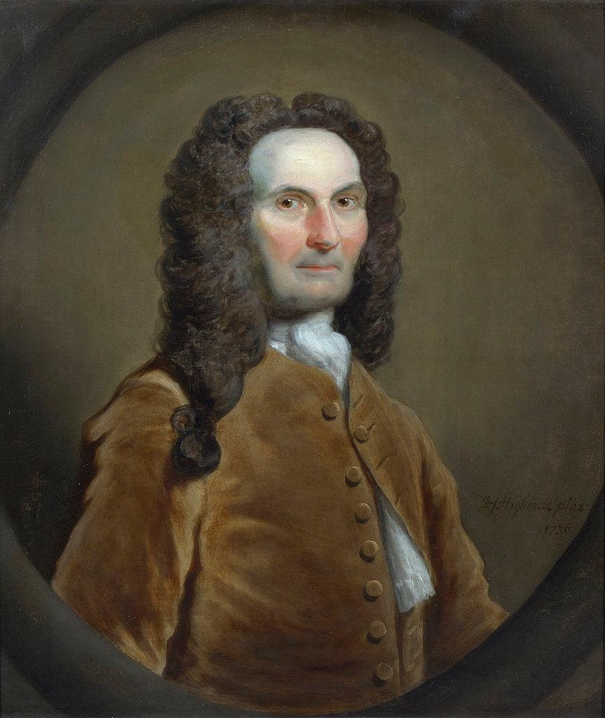
Abraham de Moivre(1667—1754)
A French-born mathematician who later spent much of his life in Britain. In addition to probability, he studied trigonometric analysis and the mathematics of annuities.
In 1733, he wrote the Latin paper Approximatio ad Summam Terminorum Binomii on sums of terms in high powers of a binomial. An English version appeared in the second edition of The Doctrine of Chances in 1738.
The problem de Moivre faced was very concrete.
In the expansion of a high power of a binomial, we can write every term exactly:
(a+b)^n
=
\sum_{k=0}^n\binom nk a^kb^{n-k}.
But when n is large, calculating the sum of many neighboring terms becomes very difficult.
And probability problems frequently require exactly this kind of summation.
For example, when p=1/2,
P(a\le S_n\le b)
=
2^{-n}\sum_{k=a}^b\binom nk.
In his 1733 work, de Moivre investigated how a continuous mathematical expression could approximate these sums of binomial coefficients. His main early breakthrough concerned the symmetric binomial distribution; Laplace later extended the underlying ideas considerably. 〔22, 23, 24〕
We will now follow his central idea and reconstruct the derivation using modern asymptotic analysis.
3.2.1 Begin with the Central Term
To simplify the notation, let
n=2m.Then
P(S_{2m}=m)
=
\binom{2m}{m}2^{-2m}
=
\frac{(2m)!}{(m!)^2\,4^m}.
Calculating the factorials directly is inconvenient.
But we can use Stirling's formula:
\boxed{
n!\sim\sqrt{2\pi n}\left(\frac ne\right)^n.
}
Here the notation
a_n\sim b_nmeans
\lim_{n\to\infty}\frac{a_n}{b_n}=1.This formula has a history well worth studying in its own right. Both de Moivre and James Stirling made important contributions to factorial asymptotics, and identifying the correct constant \sqrt{2\pi} was a crucial step. 〔25〕
Now substitute it into the central binomial coefficient.
(2m)!\sim\sqrt{4\pi m}\left(\frac{2m}{e}\right)^{2m},(m!)^2\sim 2\pi m\left(\frac me\right)^{2m}.Therefore
\begin{aligned}
P(S_{2m}=m)
&=\frac{(2m)!}{(m!)^2\,4^m}\\
&\sim
\frac{
\sqrt{4\pi m}(2m/e)^{2m}
}{
2\pi m(m/e)^{2m}4^m
}\\
&=\frac1{\sqrt{\pi m}}.
\end{aligned}
Since n=2m, we can also write
\boxed{
P(S_n=n/2)\sim\sqrt{\frac2{\pi n}}.
}
We have at last reached an important conclusion.
The probability of obtaining exactly half heads is of order
\frac1{\sqrt n}.Hence
P(S_n=n/2)\longrightarrow0.This explains the apparently contradictory phenomenon raised at the beginning of the chapter.
But the probability at the center alone does not tell us the shape of the whole distribution.
We must go on to ask:
How large are the terms a certain distance from the center, compared with the central term?
3.2.2 Moving Away from the Center
Again let n=2m.
Define
p_m(j)=P(S_{2m}=m+j).By symmetry,
p_m(j)=p_m(-j).so we need only consider j\ge0.
The relation between binomial coefficients gives
\frac{p_m(j)}{p_m(0)}
=
\frac{\binom{2m}{m+j}}{\binom{2m}{m}}.
Simplifying yields
\frac{p_m(j)}{p_m(0)}
=
\frac{m!\,m!}{(m+j)!(m-j)!}.
Expanding this further as a product,
\boxed{
\frac{p_m(j)}{p_m(0)}
=
\prod_{r=1}^j\frac{m-r+1}{m+r}.
}
This expression is intriguing.
We have transformed a ratio of enormous binomial coefficients into a product of factors close to 1.
How can we analyze the product of many numbers close to 1?
Taking logarithms is a natural choice.
Logarithms turn products into sums:
\log\frac{p_m(j)}{p_m(0)}
=
\sum_{r=1}^j
\log\left(\frac{m-r+1}{m+r}\right).
Write each term as
\log\left(1-\frac{r-1}{m}\right)
-
\log\left(1+\frac rm\right).
Now use the Taylor expansion
\log(1+x)=x-\frac{x^2}{2}+O(x^3),valid for x near 0.
Provided j does not grow too quickly relative to m, we can control all these expansions.
For j=O(\sqrt m), the leading terms after summation are
\begin{aligned}
\log\frac{p_m(j)}{p_m(0)}
&=
-\frac1m\sum_{r=1}^j(2r-1)+o(1)\\
&=-\frac{j^2}{m}+o(1).
\end{aligned}
Here we have used
\sum_{r=1}^j(2r-1)=j^2.Consequently,
\frac{p_m(j)}{p_m(0)}
\sim e^{-j^2/m}.
Combining this with the approximation to the central term,
p_m(0)\sim\frac1{\sqrt{\pi m}},we finally obtain
\boxed{
P(S_{2m}=m+j)
\sim
\frac1{\sqrt{\pi m}}e^{-j^2/m}
}
where j=O(\sqrt m). More precisely, the approximation errors can be controlled uniformly over any fixed central window |j|\le C\sqrt m.
Here a completely new functional form suddenly appears:
e^{-j^2/m}.We did not assume a normal distribution.
We have not even discussed continuous probability densities.
The squared term in the exponent arises naturally from the structure of binomial coefficients and the Taylor expansion of the logarithm.
This is the mathematical origin of the bell curve.
3.3 Why Must We Standardize by \sqrt n?
We have just derived
P(S_{2m}=m+j)
\approx
\frac1{\sqrt{\pi m}}e^{-j^2/m}.
An important question now arises.
If we let m\to\infty while keeping j fixed, then
\frac{j^2}{m}\to0.and therefore
e^{-j^2/m}\to1.This means that, for fixed j, the probabilities at different positions near the center gradually become almost equal.
We would then lose sight of the distribution's actual shape.
We must therefore find the right scale of observation.
Look at the exponent
\frac{j^2}{m}.If it is to retain nontrivial variation as m\to\infty, we should take
j\asymp\sqrt m.This is why the square-root scale appears naturally.
It does not come from knowing the definition of standard deviation in advance, or from trying to force a normal distribution to appear.
It comes from the fact that only at this scale do the relative probabilities near the center of the binomial distribution have a nontrivial limiting shape.
Now define
Z_n=\frac{S_n-n/2}{\sqrt n/2}.This subtracts the expected number of successes and divides by the standard deviation.
When n=2m and S_n=m+j,
Z_n=\frac{2j}{\sqrt n}.Let
z=\frac{2j}{\sqrt n}.Then
\frac{j^2}{m}=\frac{z^2}{2}.The earlier approximation therefore becomes
P\left(Z_n=z\right)
\approx
\sqrt{\frac2{\pi n}}e^{-z^2/2},
where z must be a lattice value that Z_n can actually take.
The distance between adjacent lattice points is
\Delta z=\frac2{\sqrt n}.Thus
\begin{aligned}
P(Z_n=z)
&\approx
\frac2{\sqrt n}\cdot
\frac1{\sqrt{2\pi}}e^{-z^2/2}\\
&=\Delta z\,\varphi(z).
\end{aligned}
where
\boxed{
\varphi(z)=\frac1{\sqrt{2\pi}}e^{-z^2/2}.
}
Now the picture becomes particularly clear.
The original binomial distribution consists of discrete probability masses.
But as n\to\infty, the spacing between successive standardized values shrinks.
The probability mass at each value is approximately
\text{interval width}\times\text{height of a continuous function}.We have found that continuous function:
\varphi(z).This is the mathematical process by which the bell curve emerges from discrete probability.
3.3.1 Watching the Bell Curve Emerge
Below, the binomial probability masses for different values of n are divided by the lattice spacing and compared with the standard normal density.
Fair coin;divide each standardized point probability by the lattice spacing,to obtain comparable curve heights。
查看母稿数值表
| z | n = 16 | n = 64 | Standard normal density |
|---|---|---|---|
| -3 | 0.00366 | 0.00425 | 0.00443 |
| -2.5 | 0.01709 | 0.01742 | 0.01753 |
| -2 | 0.05554 | 0.05435 | 0.05399 |
| -1.5 | 0.1333 | 0.13044 | 0.12952 |
| -1 | 0.24438 | 0.24259 | 0.24197 |
| -0.5 | 0.34912 | 0.35134 | 0.35207 |
| 0 | 0.39276 | 0.39739 | 0.39894 |
| 0.5 | 0.34912 | 0.35134 | 0.35207 |
| 1 | 0.24438 | 0.24259 | 0.24197 |
| 1.5 | 0.1333 | 0.13044 | 0.12952 |
| 2 | 0.05554 | 0.05435 | 0.05399 |
| 2.5 | 0.01709 | 0.01742 | 0.01753 |
| 3 | 0.00366 | 0.00425 | 0.00443 |
The lines connecting discrete lattice points in the figure serve only as a visual comparison; they do not mean that the binomial distribution itself has a continuous density.
As n increases, the correctly standardized discrete probability masses approach the same continuous function.
There is another point worth noticing.
We have not changed the coin itself.
Every toss still has only two outcomes: heads and tails.
The continuous bell curve is not the shape of an individual random experiment. It is a limiting structure that emerges when many discrete random outcomes are added and rescaled.
3.4 From Sums of Binomial Coefficients to Integrals
We now have a local approximation:
P(Z_n=z_{n,k})
\approx
\Delta z_n\,\varphi(z_{n,k}),
where
z_{n,k}=\frac{k-n/2}{\sqrt n/2},
\qquad
\Delta z_n=\frac2{\sqrt n}.
But de Moivre's original goal was not merely to approximate a single binomial coefficient.
He was interested in sums of many terms.
Take any fixed real numbers a<b.
We want to calculate
P(a\le Z_n\le b).By definition,
P(a\le Z_n\le b)
=
\sum_{\substack{k:\\a\le z_{n,k}\le b}}
P(Z_n=z_{n,k}).
Using the approximation just obtained,
P(a\le Z_n\le b)
\approx
\sum_{\substack{k:\\a\le z_{n,k}\le b}}
\varphi(z_{n,k})\Delta z_n.
Now look carefully at the right-hand side.
Does it look familiar?
It is precisely a Riemann sum.
As n\to\infty,
\Delta z_n=\frac2{\sqrt n}\to0.We should therefore obtain
\boxed{
\lim_{n\to\infty}P(a\le Z_n\le b)
=
\int_a^b
\frac1{\sqrt{2\pi}}e^{-z^2/2}\,dz.
}
This is the de Moivre–Laplace limit theorem for symmetric Bernoulli random variables.
A point about rigor is necessary here.
An approximation near each fixed location does not, by itself, justify interchanging an infinite sum and a limit.
What we need is for the relative errors in the local probability approximation to tend to zero uniformly over the fixed standardized interval [a,b].
The asymptotic expansion obtained earlier over the range |j|\le C\sqrt n provides exactly this control.
The limit can therefore be deduced rigorously from the Riemann sums.
3.4.1 Why Does the Normal Density Integrate to 1?
We have not yet explained why
\frac1{\sqrt{2\pi}}is the correct normalizing constant.
For \varphi to be a probability density, it must satisfy
\int_{-\infty}^{\infty}\varphi(x)\,dx=1.We therefore need to calculate
I=\int_{-\infty}^{\infty}e^{-x^2/2}\,dx.This integrand has no elementary antiderivative, but the definite integral can be evaluated exactly.
Consider
I^2
=
\int_{\mathbb R^2}
e^{-(x^2+y^2)/2}\,dx\,dy.
We have moved from one dimension to two.
Switch to polar coordinates:
x=r\cos\theta,
\qquad
y=r\sin\theta.
The Jacobian is r, so
\begin{aligned}
I^2
&=
\int_0^{2\pi}\int_0^\infty
e^{-r^2/2}r\,dr\,d\theta\\
&=2\pi\left[-e^{-r^2/2}\right]_0^\infty\\
&=2\pi.
\end{aligned}
Therefore
I=\sqrt{2\pi}.and hence
\boxed{
\int_{-\infty}^{\infty}
\frac1{\sqrt{2\pi}}e^{-x^2/2}\,dx=1.
}
We can finally answer one of the questions from the beginning of the chapter:
Why does \pi appear in the limiting distribution of coin tosses?
Because the asymptotic structure of binomial coefficients near their center produces an exponential of a quadratic, and the normalization of this function is closely tied to circular symmetry in two-dimensional Euclidean space.
Pi is not a physical property of the coin.
It is a geometric constant of the continuous mathematical structure we ultimately encounter.
This is a beautiful unification within probability theory:
Through limits, finite combinatorics leads to calculus; geometric symmetry within the integral then determines the normalizing constant of the probability distribution.
3.5 Laplace: Why Should the Bell Curve Belong Only to Coins?
We have now understood a special result:
\frac{S_n-n/2}{\sqrt n/2}
\xrightarrow{d}N(0,1).
Here N(0,1) denotes the standard normal distribution, and \xrightarrow d denotes convergence in distribution.
But an even more exciting question arises:
Why should we study only heads and tails?
Suppose we roll dice instead of tossing coins.
Or observe temperature errors each day.
Or study the total error produced by the accumulation of many small disturbances.
The distributions of these individual random variables may be very different from a symmetric binomial distribution.
Will their standardized sums still approach the same bell curve?
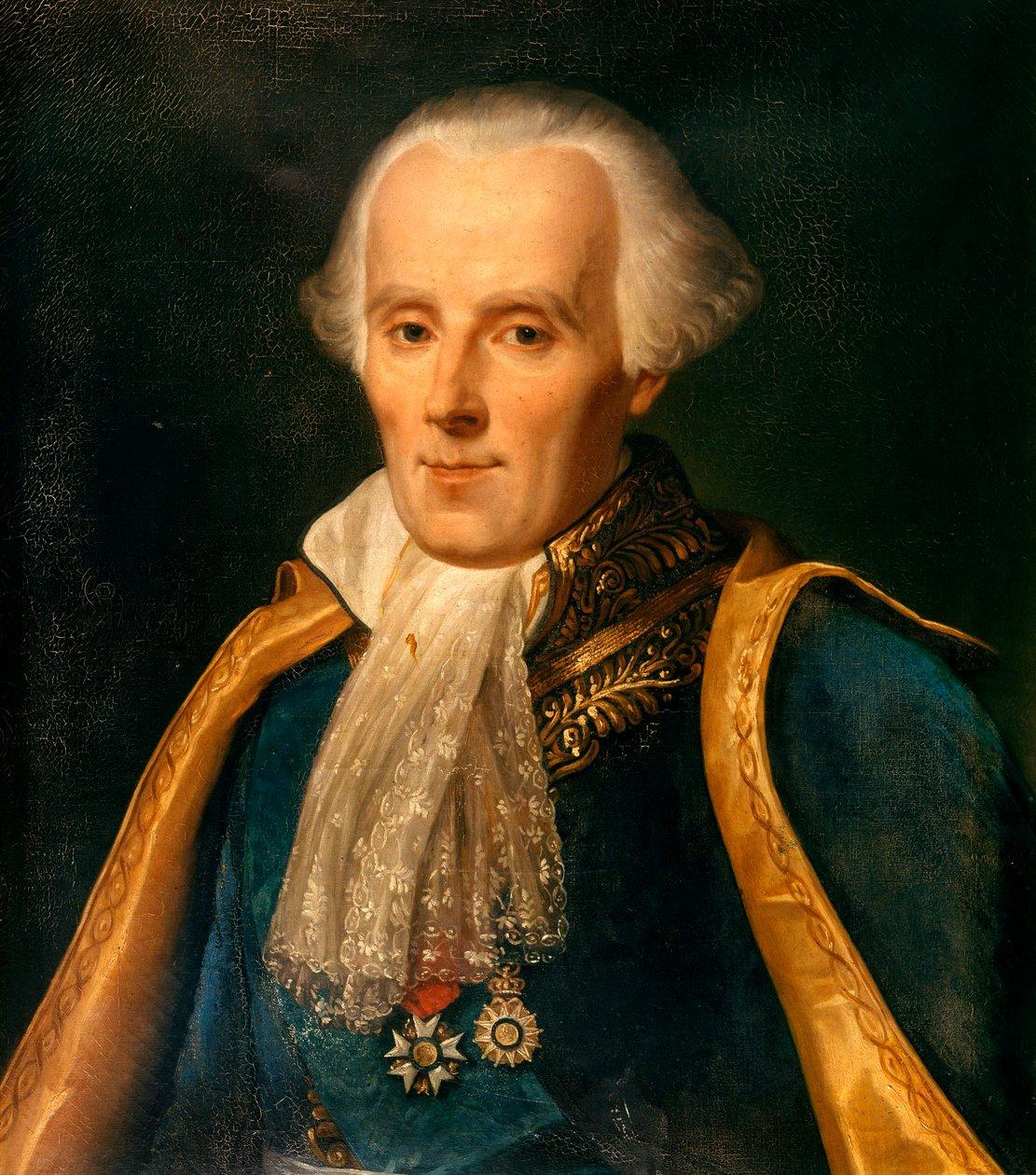
Pierre-Simon Laplace(1749—1827)
A French mathematician and astronomer.
Laplace developed probability calculations into a more general analytical theory. In particular, in his work around 1810 and in Théorie analytique des probabilités, published in 1812, he studied approximations to random sums far more general than those arising from the symmetric binomial distribution.
The passage from de Moivre's special approximation to a general central limit theorem involved a long mathematical development, rather than a simple change of symbols. Laplace's work was a pivotal part of that history. 〔26, 27, 28〕
We now study this extension in modern mathematical language.
Let
X_1,X_2,\ldotsbe independent, identically distributed random variables, and assume
\mathbb E[X_i]=\mu,0<\operatorname{Var}(X_i)=\sigma^2<\infty.They may be discrete or continuous.
Their distribution may be symmetric or skewed.
We do not assume that they have a bell-shaped density.
Now define
S_n=X_1+\cdots+X_n.By linearity of expectation,
\mathbb E[S_n]=n\mu.By independence,
\operatorname{Var}(S_n)=n\sigma^2.The most natural standardization is therefore
Z_n=\frac{S_n-n\mu}{\sigma\sqrt n}.The same \sqrt n appears here as in the coin-tossing problem.
This already suggests a more general structure.
Under these assumptions, the modern Lindeberg–Lévy central limit theorem tells us that
\boxed{
\frac{S_n-n\mu}{\sigma\sqrt n}
\xrightarrow{d}N(0,1).
}
Take a moment to appreciate this conclusion.
Each X_i on the left may have any of a wide variety of distributional shapes.
Yet after independent summation, centering, and standardization, their limiting distribution is the same N(0,1).
This is universality in a substantive probabilistic sense.
In a sense, the accumulation of many random influences makes the final distribution lose much of the detail about the individual influences.
In the independent, identically distributed model with finite variance, the scale information retained by the limit is primarily determined by the mean and variance.
Why does this happen?
We must still explain the mechanism.
3.6 The Central Limit Theorem's Real Secret: Why Do the Details of a Distribution Disappear?
Editorial supplement: Appendix D controls the remainder in the second-order expansion of the characteristic function; no third-moment assumption is added here.
We already know how to derive the normal distribution from the binomial expansion.
But if X_i have an entirely different distribution, the binomial-coefficient method no longer applies.
We need a new mathematical language.
This problem will lead us to the deep connection between probability theory and Fourier analysis.
3.6.1 Why Study Complex Exponentials?
Suppose the distribution of a random variable X is very complicated.
Studying the distribution of its independent sum
S_n=X_1+\cdots+X_ndirectly usually involves repeated convolution.
For example, if X,Y are independent with densities f_X,f_Y, then
f_{X+Y}(z)
=
\int_{\mathbb R}f_X(x)f_Y(z-x)\,dx.
For n random variables, we must convolve repeatedly.
This is a fairly complicated operation.
But mathematicians had already found in other settings that certain functional transforms turn complicated operations into simple algebra.
Define the characteristic function of a random variable X by
\boxed{
\phi_X(t)=\mathbb E[e^{itX}],
\qquad t\in\mathbb R.
}
The definition may seem rather unexpected.
Why introduce the imaginary unit i?
Why choose the exponential function in particular?
Because it has a very useful property:
e^{it(x+y)}=e^{itx}e^{ity}.Thus, if X,Y are independent,
\begin{aligned}
\phi_{X+Y}(t)
&=\mathbb E[e^{it(X+Y)}]\\
&=\mathbb E[e^{itX}e^{itY}]\\
&=\mathbb E[e^{itX}]\mathbb E[e^{itY}]\\
&=\phi_X(t)\phi_Y(t).
\end{aligned}
and consequently
\boxed{
\phi_{X+Y}(t)=\phi_X(t)\phi_Y(t).
}
We have turned addition of random variables into multiplication of characteristic functions.
The idea resembles our earlier use of logarithms to turn products into sums:
When faced with a complicated operation, seek a representation in which its difficult structure becomes a simple algebraic relation.
Dependencies on later theory: The following is a reconstruction of historical results in modern language, not de Moivre's or Laplace's original proof. Appendix D controls the remainder in the second-order expansion; Chapter 6 develops integration for complex-valued random variables; Chapter 11 systematically prove uniqueness of characteristic functions and Lévy's continuity theorem. Chapter 7 first distinguishes the relevant notions of convergence. This section continues the story through products and second-order terms, without presenting these outside results as if they had been proved here.
3.6.2 Proving the Central Limit Theorem Again with Characteristic Functions
Let
Y_i=\frac{X_i-\mu}{\sigma}.Then
\mathbb E[Y_i]=0,
\qquad
\mathbb E[Y_i^2]=1.
The standardized random sum can be written as
Z_n=\frac1{\sqrt n}\sum_{i=1}^nY_i.We now examine the characteristic function of Y_i near t=0.
Using
e^{ity}=1+ity-\frac{t^2y^2}{2}+\cdots,we expect
\phi_Y(t)
=
1+it\mathbb E[Y]
-\frac{t^2}{2}\mathbb E[Y^2]
+o(t^2).
Since the mean is 0 and the variance is 1,
\boxed{
\phi_Y(t)=1-\frac{t^2}{2}+o(t^2).
}
We do not need to assume that Y has a third moment.
A finite second moment suffices for this expansion. A rigorous proof can use
\frac{e^{iu}-1-iu}{u^2}\longrightarrow-\frac12and the corresponding boundedness to control the expectation and obtain the second-order expansion.
Now, because Y_1,\ldots,Y_n are independent,
\begin{aligned}
\phi_{Z_n}(t)
&=
\prod_{i=1}^n
\phi_{Y_i}\left(\frac{t}{\sqrt n}\right)\\
&=
\left[
\phi_Y\left(\frac{t}{\sqrt n}\right)
\right]^n.
\end{aligned}
Using the Taylor expansion above,
\phi_Y\left(\frac{t}{\sqrt n}\right)
=
1-\frac{t^2}{2n}+o\left(\frac1n\right).
Therefore
\phi_{Z_n}(t)
=
\left[
1-\frac{t^2}{2n}+o\left(\frac1n\right)
\right]^n.
Recall the elementary limit
\left(1+\frac an+o\left(\frac1n\right)\right)^n
\longrightarrow e^a.
It follows that
\boxed{
\lim_{n\to\infty}\phi_{Z_n}(t)
=
e^{-t^2/2}.
}
But
e^{-t^2/2}is precisely the characteristic function of a standard normal random variable.
The continuity theorem for characteristic functions therefore gives
\boxed{Z_n\xrightarrow d N(0,1).}This completes the proof.
This modern proof differs from de Moivre's and Laplace's original derivations, but reveals the central mathematical mechanism of the central limit theorem.
3.6.3 Why Does Only the Second-Order Term Survive?
Look again at
\phi_Y(t)=1-\frac{t^2}{2}+o(t^2).When standardizing the sum, we replace t by t/\sqrt n.
The second-order term becomes
\frac{t^2}{n}.Multiplying the characteristic functions of n independent random variables produces a nontrivial limit:
n\cdot\frac{t^2}{n}=t^2.Under suitable moment conditions, the higher-order terms gradually disappear.
For example, if the third moment exists, the accumulated third-order contribution is of order
n\left(\frac t{\sqrt n}\right)^3
=
\frac{t^3}{\sqrt n}
\to0.
The fourth-order term gives
n\left(\frac t{\sqrt n}\right)^4
=
\frac{t^4}{n}
\to0.
Thus only the second-order structure survives in the limit.
This explains why independent sums from many different distributions have the same limit.
We do not need to know every detail of each distribution.
At this limiting scale, many higher-order details become invisible.
And the characteristic function supplied by the second-order term,
e^{-t^2/2}corresponds precisely to the normal distribution.
The central limit theorem therefore does much more than happen to announce that sums of many random variables “look bell-shaped.”
It expresses the following mathematical principle:
Independent summation and square-root standardization preserve second-order structure in the limit while diminishing other local details.
This is a central reason for the universality of the normal distribution.
3.7 Gauss: Why Do Astronomers Also Encounter the Bell Curve?
So far, we have discovered the normal distribution by following a path through gambling, binomial expressions, and independent random sums.
Historically, another important path led to the same function.
It began not with dice,
but with measurement errors in astronomy.
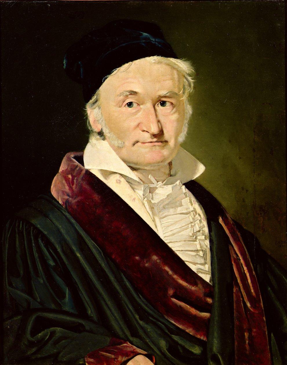
Carl Friedrich Gauss(1777—1855)
A German mathematician and astronomer.
In Theoria Motus Corporum Coelestium (1809), he discussed celestial orbits and observational errors, and established an important connection between normally distributed errors and least-squares estimation.
Legendre had already published the method of least squares in 1805; Robert Adrain independently studied the normal law of errors in 1808. Simply attributing the discovery of the normal distribution to Gauss alone therefore misrepresents its mathematical history. 〔27, 29, 30〕
Yet Gauss's argument contains an idea that deserves close attention:
Why, when repeatedly measuring the same unknown quantity, do we tend to use the arithmetic mean as an estimate?
For example, suppose we measure an unknown length \theta and obtain
Y_1,\ldots,Y_n.Assume
Y_i=\theta+\varepsilon_i,where \varepsilon_i are measurement errors.
The mathematician wants to recover \theta from these imperfect observations.
A natural method is to average:
\widehat\theta=\frac1n\sum_{i=1}^nY_i.But why should the average be the right estimate?
Can we reverse the question?
If we require the arithmetic mean to be the most likely estimate, what form must the probability distribution of the errors take?
Reading route: Returning to Gauss's problem of errors and estimation gives another historical source of the Gaussian law; it does not imply that Gauss worked after the modern characteristic-function proof. The functional-equation argument below is a modern reconstruction. The linearity of measurable additive functions remains a tool to be supplied later, and the related regularity questions are retained in the review issue register.
3.7.1 Recovering a Probability Distribution from an Optimal Estimate
Assume the errors \varepsilon_i are independent and identically distributed, with an everywhere positive, differentiable density f.
Given observations y_1,\ldots,y_n, the likelihood function for the parameter \theta is
L(\theta)=\prod_{i=1}^n f(y_i-\theta).We now impose a strong assumption:
Whatever the sample and whatever its size, the arithmetic mean
\overline y=\frac1n\sum_{i=1}^ny_ishould be a maximum likelihood estimate.
Let us see what constraints this places on the density f.
For convenience, let
\psi(x)=\frac{f'(x)}{f(x)}.Differentiate the log-likelihood:
\frac{d}{d\theta}\log L(\theta)
=
-\sum_{i=1}^n\psi(y_i-\theta).
If the maximum occurs at \theta=\overline y, the first-order condition requires
\sum_{i=1}^n\psi(y_i-\overline y)=0.Let
r_i=y_i-\overline y.Notice that
\sum_{i=1}^nr_i=0.Our assumption therefore implies that
for every set of residuals satisfying \sum r_i=0, we have
\boxed{\sum_{i=1}^n\psi(r_i)=0.}First consider n=2.
Taking residuals x,-x gives
\psi(x)+\psi(-x)=0.Thus \psi is odd.
Next consider n=3.
Take the residuals
x,\quad y,\quad -(x+y).Then
\psi(x)+\psi(y)+\psi(-(x+y))=0.Using oddness,
\boxed{
\psi(x+y)=\psi(x)+\psi(y).
}
This is Cauchy's functional equation!
Under a suitable regularity assumption, such as continuity, we have
\psi(x)=cxfor some constant c.
But since
\psi(x)=\frac{f'(x)}{f(x)},we obtain
\frac{d}{dx}\log f(x)=cx.Integrating gives
\log f(x)=\frac c2x^2+C.and hence
f(x)=Ae^{cx^2/2}.For f to be an integrable probability density on the whole real line, we must have
c<0.Let
c=-\frac1{\sigma^2},Then
f(x)=Ae^{-x^2/(2\sigma^2)}.Normalization gives
\boxed{
f(x)=
\frac1{\sqrt{2\pi}\sigma}
e^{-x^2/(2\sigma^2)}.
}
Once again, we have obtained the normal density!
This time, however, it did not arise as a limit of binomial coefficients.
It arose from a requirement on an estimation method:
In the independent, identically distributed error model above, under the stated regularity conditions, requiring the arithmetic mean to be a maximum likelihood estimate for every sample leads to normally distributed errors.
This is a modern reconstruction of Gauss's line of reasoning in 1809. It does not prove that all real-world observational errors are normally distributed; it shows a special relationship between a certain optimality requirement for the average and the normal model. 〔30〕
Going further, we can understand why least squares is so closely connected with the normal distribution.
In the normal error model, apart from constants independent of \theta and a positive scaling factor, the negative log-likelihood is precisely
\sum_{i=1}^n(y_i-\theta)^2.Maximizing the likelihood is the same as minimizing the squared error.
Thus
\boxed{
\text{normal error model}
\Longrightarrow
\text{least squares and maximum likelihood are connected}.
}
Mathematical methods that arose historically from different problems acquire a unified explanation here.
3.8 Must Every Random Phenomenon Eventually Become Normally Distributed?
By this point, the normal distribution may seem capable of everything.
The sum of coin tosses approaches a normal distribution.
Standardized sums of general independent random variables also approach a normal distribution.
The analysis of measurement errors again produces the normal density.
Should we conclude that the normal distribution is the inevitable final form of random phenomena?
No.
The central limit theorem has very specific assumptions.
When those assumptions fail, its conclusion may be entirely different.
Let us consider a particularly important example.
Dependencies on later theory: This example still uses as known results the characteristic-function formula and the identification of distributions by characteristic functions. The calculation and uniqueness theory are scheduled for Chapter 11; presenting a counterexample here does not mean that the corresponding theory has already been established.
3.8.1 The Cauchy Distribution: A Random Variable That Averaging Cannot Tame
Let
X_1,X_2,\ldotsbe independent and identically distributed, each with the standard Cauchy distribution:
f(x)=\frac1{\pi(1+x^2)}.Its characteristic function is
\phi_X(t)=e^{-|t|}.Now calculate the sample average
\overline X_n=\frac1n\sum_{i=1}^nX_i.Using characteristic functions and independence,
\begin{aligned}
\phi_{\overline X_n}(t)
&=
\prod_{i=1}^n
\phi_X\left(\frac tn\right)\\
&=
\left(e^{-|t|/n}\right)^n\\
&=e^{-|t|}.
\end{aligned}
This is exactly the characteristic function of a single X_i.
Consequently,
\boxed{
\overline X_n\overset d=X_1
}
for every n\ge1.
This means that
no matter how many independent standard Cauchy random variables we average, the distribution of the average does not become more concentrated.
It remains standard Cauchy.
The usual convergence conclusion of the law of large numbers fails here, and the standard central limit theorem with finite variance certainly does not apply.
The reason is that the Cauchy distribution has neither a finite first absolute moment nor a finite variance.
We now see that
the universality of the normal distribution is conditional.
It depends on the tail behavior of the random variables, their dependence structure, and the scale chosen for summation.
When these conditions change, the limit may belong to a completely different family of distributions.
This leads to stable distributions, generalized central limit theorems, and modern probability theory's study of heavy tails.
It also shows that the normal distribution is the starting point of a broader theory of random limits, rather than the endpoint of randomness.
Chapter 3 Conclusion: What Have We Really Discovered?
Let us retrace the chapter's line of thought.
At the outset, we had a very concrete difficulty:
calculating
2^{-n}\sum_{k=a}^{b}\binom nkbecomes exceedingly troublesome when n is large.
To understand it, we studied the central term and then compared neighboring binomial coefficients.
Taking logarithms and applying a Taylor expansion brought out
e^{-x^2/2}.To obtain a nontrivial limiting shape, we had to introduce a scale such as \sqrt n.
As the discrete lattice spacing tends to zero, sums of binomial coefficients become integrals.
The bell curve then emerges naturally.
The direction of generalization advanced by Laplace next tells us that this limiting phenomenon extends beyond binomial distributions.
Modern characteristic functions reveal the structure behind it:
\left(
1-\frac{t^2}{2n}
+o\left(\frac1n\right)
\right)^n
\longrightarrow e^{-t^2/2}.
After independent summation and suitable standardization, a complicated random system exhibits a universal limiting form determined by second-order structure.
Meanwhile, Gauss's analysis of measurement errors reveals connections between the normal distribution and the optimality of the arithmetic mean and least squares.
Two quite different paths of inquiry finally meet.
Adding Many Random Events de Moivre → Laplace
\sum X_iMeasurement Errors and Optimal Estimation Legendre → Gauss
\min_\theta\sum(Y_i-\theta)^2The Normal Distribution
f(x)=\frac{1}{\sigma\sqrt{2\pi}}e^{-\frac{(x-\mu)^2}{2\sigma^2}}Probabilistic limits, analytical structure, and statistical estimation come together here.
But I believe this chapter contains an idea more important than any individual formula.
We have found two phenomena that initially seem entirely opposed:
On the one hand, random events produce unpredictable fluctuations.
On the other, after enough accumulation, those fluctuations exhibit a stable and universal mathematical regularity.
This does not mean that the world has ceased to be random.
Quite the contrary.
By studying randomness itself carefully, mathematicians discovered the order that randomness allows.
We can now explain why random errors from different sources may produce approximately the same bell curve.
Yet another question arises.
In our earlier study of random variables, we could often begin by explicitly writing down their probability distributions.
But many random objects in the real world vary continuously.
For example, a particle keeps moving in a liquid.
We want to know not only its position at a particular time, but also how it moves randomly over an entire time interval.
More puzzling still:
If we observe this motion on shorter and shorter time scales, what will we ultimately see?
As the time interval tends to zero, can we construct a mathematical process that is truly continuous yet remains random throughout?
This will force us to move from individual random variables to stochastic processes consisting of infinitely many random variables.
It will also bring us back to a question that first appeared in Chapter 1:
When the possible random outcomes form an infinite and complicated space, how should we define probability?
This prepares the way for our journey into measure theory, stochastic processes, and Brownian motion.
Coming Next
Chapter 4: When Randomness Enters Time—From Random Walks to Brownian Motion
We will begin with a very simple model:
S_n=X_1+\cdots+X_n,
\qquad P(X_i=1)=P(X_i=-1)=\frac12.
Then we will ask:
Why, after shrinking space by 1/\sqrt n and time by 1/n, can a random motion that jumps on an integer lattice converge to a stochastic process with continuous paths?
This will be our first real encounter with random functions themselves, beyond random numbers alone.
It will also provide another important foundation for our later study of random trees, the CRT, and continuous random geometry.
The Mathematics of Chance · Volume I, Chapter 3 · Working Draft v0.1