Chapter 25: When Does a Random Walk Become Brownian Motion?—Donsker’s Invariance Principle

An observer records a random walk at increasingly frequent times and asks whether the particle ever crossed a fixed horizontal level. Looking only at the last photograph misses earlier crossings; a few extra photographs can still miss motion between them. The spikes in Chapter 23 exposed this difficulty. We must now decide whether the walk’s own increments can rule it out.

Brownian motion already exists as a probability law on continuous paths. The task is no longer to imagine a limiting curve, but to prove that discrete records approach its path law. The remarkable point is that independence, identical distribution and a finite variance still suffice. Understanding that “still” requires taking seriously steps that are large but infrequent.

25.1 What the one-dimensional theorem never promised

Let centered increments ξᵢ be iid with mean zero and variance one, and let Sₖ be their partial sums. The central limit theorem controls Sₙ/√n; its multivariate version controls any fixed collection of times. But “crossed at some time” involves all times. The grid maximum makes the distinction visible: the dimension grows with n instead of remaining fixed.

A limit valid in every fixed dimension cannot simply be applied to an event whose dimension keeps growing. Chapter 24 named the missing ingredient tightness: most curves must obey control at a common time resolution. Rather than prove Prokhorov again, we must obtain that control from the structure of independent sums.

25.2 Specify what is being magnified

For original steps Yᵢ with mean μ and variance σ²∈(0,∞), first set ξᵢ=(Yᵢ−μ)/σ. This removes deterministic mean drift, not the realized average of that particular sample. The latter would force the path back to zero and produce a different limit. We use mean zero and variance one first and restore units afterward.

Wₙ retains the value after each recorded step and is a right-continuous staircase; Lₙ joins neighboring records linearly. They agree at every grid point. The time step 1/n and spatial scale 1/√n are linked: about nt steps have variance nt, and division by n leaves t, the Brownian covariance time scale.

On [0,T] both paths depend on finitely many increments. Linear interpolation is continuous from that vector into C([0,T]); fixed-grid step interpolation is continuous in uniform norm and hence in J₁. Thus these are C-valued and D-valued random elements. Half-line measurability follows from the finite windows and coordinate Borel structures, not from an unsupported identification of separate coordinate measurability with path measurability.

25.3 Exactly how far apart are the interpolations?

Within a grid cell the line traverses that cell’s increment while the step remains at its left value. The discrepancy is therefore bounded by the largest step in the observation window. This is more precise than saying that steps look small: increments are random and their maximum must be controlled.

A finite second moment suffices. For ε>0 the union bound and the tail second moment give the estimate below. Merely applying Markov’s inequality would give a constant bound; the growing threshold inside the indicator makes the tail integral actually vanish.

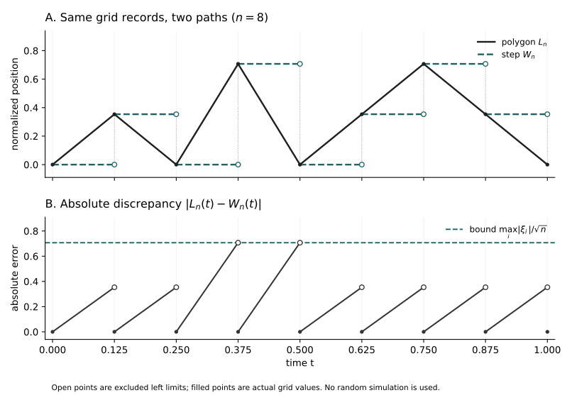
The interpolations become close in probability, but neither has yet been proved to have a path limit. If Lₙ hid spikes like those in Chapter 23, both approximations could fail together. The maximum-step estimate resolves interpolation choice, not all of tightness.

25.4 How the Gaussian finite-dimensional laws appear together

Take 0=t₀<t₁<⋯<tₘ. First examine increments over disjoint intervals rather than positions. Interval j contains mₙⱼ=⌊ntⱼ⌋−⌊ntⱼ₋₁⌋ original increments. Every time gap is positive, so all mₙⱼ>0 for sufficiently large n, as required by the normalization below. Each block is an independent sum and distinct blocks are independent. This is what permits a joint limit from the one-dimensional CLT.

By the finite-variance CLT of Chapter 11 and multivariate characteristic-function tools of Chapter 14, the block vector has a product characteristic function. For arbitrary real θ₁,…,θₘ its limit is below. The multivariate continuity theorem identifies independent Gaussian blocks. A continuous linear cumulative-sum map then gives the joint law of positions.

These are precisely the finite-dimensional distributions of Brownian motion constructed in Chapter 23, with position covariance min(s,t). The previous section makes the differences between Lₙ and Wₙ vanish simultaneously at finitely many coordinates, so the polygons share the limit. We have not reproved the CLT; the new task was to identify independent time blocks and connect them to the path problem.

25.5 Why the variance estimate stops at the threshold

Trying to use Chapter 24’s uniform increment-moment criterion reveals a genuine obstruction. On the grid the variance has only the first power of the time gap, whereas that criterion requires a power greater than one so that estimates can be summed over increasingly many grid edges. A small average squared increment has not automatically become uniform continuity control for a family.

A fourth moment would temporarily give an additional time power through independence. Keeping that convenient assumption permanently would exclude many walks that should have Brownian limits. For example the symmetric density below has mean zero and variance one but no fourth moment.

The density integrates to one; symmetry and a finite first moment give mean zero. With u=1+x the second tail integral is 2∫₁∞(u⁻²−u⁻³)du=1, while the fourth-moment tail integrand 4x³/(1+x)³ does not tend to zero and its integral diverges. The issue is not a lack of examples but how a proof can cross the fourth-moment threshold.

25.6 Let the fourth moment do its proper job first

First suppose centered iid steps ηᵢ have second moment v and fourth moment m₄. The polygonal increment from s to t is a weighted sum of independent steps. The coefficient aᵢ is the fraction of its cell lying in [s,t]; it belongs to [0,1], and the coefficients sum to n(t−s).

After expanding the fourth power, every term with an index appearing only once vanishes by centering and independence. Only fourth powers and paired terms remain. The identity explains where the additional time power comes from.

Put u=n(t−s). For u≥1, Σaᵢ⁴≤u≤u² and Σaᵢ²≤u. For u≤1, Σaᵢ⁴≤u⁴≤u² and (Σaᵢ²)²≤u⁴≤u². The latter case cannot be omitted: s and t may lie inside one cell. Together the cases give a uniform bound at all real times.

Chapter 24’s moment criterion with α=4 and β=1, together with the zero starting value, yields tightness in C([0,T]). Finite-dimensional laws identify √v B, with the zero process when v=0. The fourth-moment route is complete, but remains one component of the truncation argument.

25.7 Truncation does not pretend large steps are absent

Fix K>0 and split ξ into a bounded centered part and a remainder. Centering must be adjusted too. A zero original mean does not force the truncated mean to vanish; even a small fixed mean, added n times and divided by √n, produces an increasing drift.

For each fixed K the truncated increments have finite fourth moments, so the previous section makes their polygons Lₙ⁽ᴷ⁾ tight. Their variances approach one because the remainder tends to zero in L². We need not exchange the limits in K and n: first show that the remainder path is small on the whole window.

Bounding the sum of absolute remainders would destroy cancellation from centering and often leave √n times a first-order tail quantity. Kolmogorov’s maximal inequality from Chapter 12 controls the remainder partial sums while preserving independence and zero means.

The first step uses only that a line segment is a convex combination of its endpoints. The maximal inequality requires independent centered summands with finite variance, not fourth moments and not independence between a truncated part and its remainder. Those two parts are usually dependent, and no such additional assumption is used.

25.8 Put the two limits in the right order

Let w be the continuous-path modulus from Chapter 24. Two curves within uniform distance a have moduli differing by at most 2a. A bad modulus for the original path is therefore covered by a bad modulus for its truncated version and a large remainder-path event.

The right side is valid for every fixed K. First let δ decrease to zero, using fourth-moment tightness for that K; then let K increase to infinity, removing the tail second moment. The starting point is zero and finitely many initial indices can be included by their individual continuity. Thus the laws of Lₙ are uniformly tight in C([0,T]).

The fourth-moment constant may grow rapidly with K or diverge. That does not hurt the proof: it is uniform in n for a fixed K, not uniform in K. Choosing a truncation level depending on n and silently treating this constant as uniform would conceal the argument’s crucial quantifier order.

25.9 Donsker’s theorem now becomes a path theorem

We can now complete the main result. If ξᵢ are iid with Eξ₁=0 and Eξ₁²=1, the law of Lₙ converges weakly in C([0,T]) to the restricted standard Brownian law for every T<∞.

All pieces are now present. Section 25.4 gives the finite-dimensional limit; Sections 25.6–25.8 give tightness. Chapter 24’s identification theorem makes every subsequential weak limit the Wiener measure already constructed in Chapter 23, and the bad-subsequence argument recovers the whole sequence. Brownian existence did not depend on Donsker, so the claimed limit is not being used to construct itself.

For general Yᵢ, subtract μnt from the polygonal partial sum and divide by σ√n. A constant increment μ accumulates exactly to μnt under linear interpolation, so no grid-centering error appears. If σ=0 then Yᵢ=μ almost surely and the centered path is zero; the nondegenerate Brownian version explicitly requires σ>0.

25.10 Steps, polygons and growing observation windows

Wₙ does not belong to C, so it cannot be said to converge in C. The continuous inclusion C→D transfers the limit of Lₙ to J₁ space. Since J₁ distance is bounded by truncated uniform distance, the discrepancy in Section 25.3 and the stability result of Chapter 24 give the same D-valued limit for Wₙ.

The tightness proof was completed entirely in C without using Aldous’s criterion. The logarithmic-clock and coordinate-generation proofs of the Polish and Borel facts are in T-J1; here we use its measurable structure, continuous inclusion and distance control. The Brownian limit is continuous, and the interpolation discrepancy already vanishes in the stronger uniform distance.

On the half-line, apply the argument to each integer window and then use Chapter 24’s C_loc tightness and finite-dimensional identification to get Lₙ⇒B in C_loc. The steps converge in real half-line local J₁ as well. In T-J1’s integral metric, the uniform-distance bound vanishes in probability on each fixed window; boundedness makes its expectation vanish, Tonelli and dominated convergence remove the window integral, and Markov gives convergence of the entire local distance in probability. This does not require every jump limit to be stable at integer endpoints; the present limit is continuous everywhere.

25.11 Which questions can a path limit carry with it?

The maximum no longer needs a growing-dimensional integral. On C([0,T]), the supremum, infimum, range and time integral are continuous; the difference of two suprema is at most their uniform distance. Continuous mapping yields a family of genuinely functional limit theorems.

Crossing probabilities still obey Portmanteau: direct convergence follows at a threshold a only when the limiting maximum has no atom there. We do not borrow Chapter 26’s reflection principle to insert a maximum distribution formula, nor treat first hitting time as an everywhere continuous map. Paths that merely touch a boundary can make first passage unstable.

Weak convergence alone does not promise convergence of expectations. Here Chapter 15’s L² maximal inequality additionally gives E max_{k≤n}|Sₖ|²/n≤4. The grid maxima themselves are uniformly integrable; truncating continuous readings and then removing the tails gives convergence of their expectations to the Brownian maximum’s expectation. This bound does not prove uniform integrability of squared maxima and cannot silently yield another moment order.

25.12 What finite variance and independence each do

Finite variance does more than provide a CLT at the final position. It makes the largest individual step disappear on the √n scale and the truncated tail negligible along the entire path. The density without a fourth moment in Section 25.5 satisfies the theorem fully. Fourth moments are a tool for bounded approximations, not an extra assumption on the original walk.

Independence controls cancellation and the joint structure of time blocks. Take independent symmetric signs εⱼ but set ξ₂ⱼ₋₁=εⱼ and ξ₂ⱼ=−εⱼ. Each step still has mean zero, variance one and absolute value one, but pairs cancel exactly. The polygon’s uniform norm is at most 1/√n and the limit is zero. A step’s marginal law and boundedness do not replace independence.

For standard Cauchy increments, Sₙ/n remains standard Cauchy while Sₙ/√n has scale √n and is not even tight at the endpoint. The stable laws of Chapter 14 show that the square-root scale, rather than the very possibility of limits, has failed. Nor must every infinite-variance model have a non-Gaussian limit: infinite-variance Gaussian domains of attraction require additional truncated-variance and scaling theory, not an automatic extension here.

25.13 Step variances approaching one can still leave large jumps

The phrase “identically distributed” carries an easily missed quantifier. The theorem uses one fixed step law, not a newly selected variance-one law whenever n changes. Chapter 13’s rare events show the difference. For each row n≥2 take independent Bernoulli(1/n) variables Iₙₖ and put ξₙₖ=√n(Iₙₖ−1/n), k=1,…,n.

The endpoint approaches Poisson(1)−1 rather than a Gaussian. More directly, on at least one success the polygon rises by 1−1/n within a cell of width 1/n. That event has probability tending to 1−e⁻¹; for every fixed δ>0 the modulus is at least 1−1/n for large n. C-tightness fails. A large jump becomes rare in any specified cell, yet retains a nonvanishing chance of occurring somewhere among all cells.

Dividing further by √(1−1/n) makes each step variance exactly one without changing the failure. This is the nonvanishing contribution of large jumps to total variance controlled by Chapter 14’s Lindeberg condition. The finite-variance invariance principle has not abolished that requirement; a fixed law’s second tail moment automatically supplies the needed control.

25.14 Why a fixed sample size leaves a bridge

Path limits apply beyond returns accumulated in time. Take iid uniform Uᵢ on [0,1] and move a threshold t from left to right, recording the sample fraction Gₙ(t) in [0,t]. Chapter 12 gives uniform convergence of Gₙ to t. Now magnify the remaining error by √n.

At t=1 the total count is fixed at n and the error is exactly zero. Counts added at different thresholds cannot be independent because they allocate the same sample. The covariance has the extra term −st. The Brownian bridge of Chapter 23 appears for a structural reason: a fixed total really changes Gaussian dependence.

Covariance alone still does not prove a process limit. We need a representation connecting the whole empirical curve to independent sums. Ordered uniform points divide the interval into random gaps; independent exponential waits, normalized by their total length, produce exactly those gaps. This exact finite-sample identity is more direct than introducing unproved empirical-process tightness machinery.

25.15 Exponential spacings turn sums into an empirical curve

Take iid exponential variables Eᵢ of mean one, with partial sums Rₖ, and let N=n+1. The vector (R₁/R_N,…,Rₙ/R_N) has the law of n uniform order statistics. The transformation Eᵢ=r(uᵢ−uᵢ₋₁) has Jacobian rⁿ, and integration gives ∫₀∞e⁻ʳrⁿdr=n!, exactly the uniform order-statistic density. T-FCLT gives the full variable ranges, Jacobian and normalization calculation.

Join Rₖ/R_N linearly at k/N to obtain a strictly increasing homeomorphism q_N. Write H_N for the centered exponential polygon. Donsker and continuous mapping give the formula below. The denominator fixes total length at one, removing the fluctuation shared with the endpoint.

The empirical CDF reverses the question: how many gaps have been traversed when the spatial threshold reaches t? It requires the inverse r_N=q_N⁻¹, satisfying √N(r_N−id)=−v_N∘r_N. Since q_N approaches the identity, so does r_N. C-tightness of v_N makes the uniform error from this small time change vanish. Thus the inverse fluctuation approaches −B°.

The empirical CDF formed from these gaps differs from r_N by at most 1/N, negligible on the √n scale. The centered Gaussian symmetry makes −B° and B° identically distributed; the minus sign cannot simply be removed when discussing joint limits with the original Brownian motion. The resulting empirical-process theorem is:

This uses D-valued random elements and a representation uniformly close to continuous processes. It does not assume Borel weak convergence in a nonseparable uniform-norm function space. The density representation, inverse error and continuous-mapping steps are all supplied in the actual T-FCLT empirical-process proof.

25.16 Reading the bridge through a different population law

For samples from a general distribution function F, write their empirical CDF as Fₙ. Chapter 7’s quantile construction represents the sample as Q_F(Uᵢ), with 1_{Q_F(Uᵢ)≤x}=1_{Uᵢ≤F(x)}. The new fluctuation is the uniform empirical process read at time F(x).

When F is discontinuous, the limit can jump at population atoms; it is not forcibly described as a continuous process. The map g↦g∘F from continuous functions is a contraction in uniform distance and produces càdlàg paths, so continuous approximations prove this version. The topological reason is that J₁ convergence to a continuous g is equivalent to uniform convergence, so the uniform error of gₙ∘F is bounded by that of gₙ and g even when F is discontinuous. The previous section’s C-valued approximations implement this limit rigorously; no continuity of composition at a general jump limit is presumed. If F is continuous the limit is continuous as well. See T-FCLT for the finite-interval statement and measurability.

The uniform case also gives √n‖Gₙ−id‖∞⇒‖B°‖∞. One path limit organizes errors at every threshold instead of repeating a normal approximation infinitely many times. We do not compute the explicit bridge-supremum distribution here; that requires separate path arguments.

25.17 How sums of waits become arrival counts

In Chapter 19 renewal counts and sums of waits were inverse questions. Let τᵢ>0 be iid with mean μ>0 and variance σ²∈(0,∞), let Rₖ=τ₁+⋯+τₖ and N(t)=max{k:Rₖ≤t}. If total waiting lies above its mean line, fewer arrivals fit into a fixed time. This visible inverse relationship accounts for the minus sign in the limit.

The result does not follow by formally differentiating an inverse. First the strong law and monotonicity give uniform convergence of N(nt)/n to t/μ on compact windows. Finite second moments then make the largest among about Cn waits negligible after division by √n, controlling the unfinished interval at the random index. Finally the common modulus of the waiting-sum process permits replacing random time N(nt)/n by t/μ. The companion renewal proof supplies every step.

The same maximum-wait estimate makes age and residual life, divided by √n, vanish uniformly on compact windows. This is negligibility at the present macroscopic scale, not their unscaled stationary limit theorem or a heavy-tailed functional renewal limit. In infinite-variance or potentially explosive models the inverse idea requires fresh scaling and continuity checks.

25.18 What is invariant, and what is not

Invariance means that under these assumptions and this scaling, different step laws share one macroscopic path law. Microscopic skewness, the presence of a density and the existence of fourth moments may differ. After centering and variance normalization, independent small fluctuations have the same path limit. This does not erase all microscopic information or make real motion automatically satisfy the assumptions.

In particular, weak convergence does not say that the original walks converge path by path to a particular Brownian trajectory. Even for iid standard normal increments, Aₙ=Sₙ/√n has A₂ₙ−Aₙ centered normal with variance 2−√2. Thus Aₙ is not Cauchy in probability. Even endpoints on the original probability space need not converge in probability, much less paths automatically converge individually.

Chapter 24’s Skorokhod representation permits almost-sure approximation on another common space, preserving each n’s marginal path law rather than the original dependence across n. Strong approximation poses further questions of its own. Keeping these conclusions separate makes the achieved universality precise.

25.19 Continuous motion emerges from the records

At first the denser photographs told us only that positions at finitely many times looked Gaussian. Independent sums now supply control beyond those photographs. The bounded part’s fourth-power expansion restrains fine oscillations, while tail second moments and a maximal inequality prevent rare large steps from ruining the entire record. Continuity of the limit is guaranteed between these two controls, not guessed from a smoothly drawn picture.

The same path viewpoint gives a pinned bridge for fixed-sample counts and count fluctuations when waiting sums are read in reverse. Path space makes connections between experiments provable: not because their pictures resemble one another, but because maps, errors and common tightness are explicitly controlled.

Continuity, however, is not smoothness. Every polygon has a slope inside each cell, but existence of a limit does not make these slopes converge to a velocity. Crossing and first passage retain boundary difficulties that continuous readings alone do not remove. Brownian motion is now both a constructed law and a shared limit of many discrete records. The next object of close observation is this very path, whose existence and approximation are now established.

25.20 Sources, proof methods and scope

Monroe Donsker’s An Invariance Principle for Certain Probability Limit Theorems appeared in Four Papers on Probability, Memoirs of the American Mathematical Society no. 6 (1951); see the official AMS record. His Justification and Extension of Doob’s Heuristic Approach to the Kolmogorov–Smirnov Theorems appeared in Annals of Mathematical Statistics 23 (1952), 277–281; see the original journal record. These sources establish historical attribution, not a claim to reproduce the original proofs or identify their function-space formulations with the later mature Borel weak-convergence framework.

The proof is a modern reconstruction: Wiener measure constructed independently in Chapter 23 is identified using Chapter 24’s path tightness. Bounded fourth moments and fixed truncation give the general finite-second-moment result; exponential spacings and inverse maps give the stated empirical and finite-variance renewal versions. The old Donsker module retains its original derivation; the general proof is now here and in T-FCLT. Brownian stopping-time embeddings, strong approximation, general empirical function classes, heavy-tailed renewal and conditioned random-tree limits are not automatically established.