Haobai Wang · Public reading edition · ch04-en-fdbc3299fbd8
This content fingerprint identifies the text, not academic final approval or an independent proof of authorship.
SHA-256: fdbc3299fbd8bb58dbc7a9021e4c3f1963519b85114704404bb55cf9053c089e
The Mathematics of Chance
Volume I · Can Chance Be Calculated?
Chapter 4: When Randomness Enters Time—From Random Walks to Brownian Motion
Can snapshots of Gaussian distributions be assembled into a genuine random path?
In Chapter 3, we discovered a profound phenomenon in probability theory.
After suitable centering and standardization, the sum of many independent random variables may converge to a normal distribution:
\frac{X_1+\cdots+X_n-n\mu}{\sigma\sqrt n}
\xrightarrow{d}N(0,1).
Until now, however, we have treated the random experiment as a whole.
We cared only about the final sum of the first n random variables.
Now suppose that, instead of observing only the final sum, we record the position of the random system at every step.
The single random variable
S_n=X_1+\cdots+X_nthen becomes an entire sequence of random variables:
S_0,S_1,S_2,\ldotsWe begin to ask a new question:
How does randomness develop over time?
This question will take probability theory beyond individual random numbers into random paths, stochastic processes, and eventually spaces of random functions.
Along the way, we will encounter one of the most important objects in modern probability theory: Brownian motion.
4.1 A Botanist Discovers a Mathematical Problem
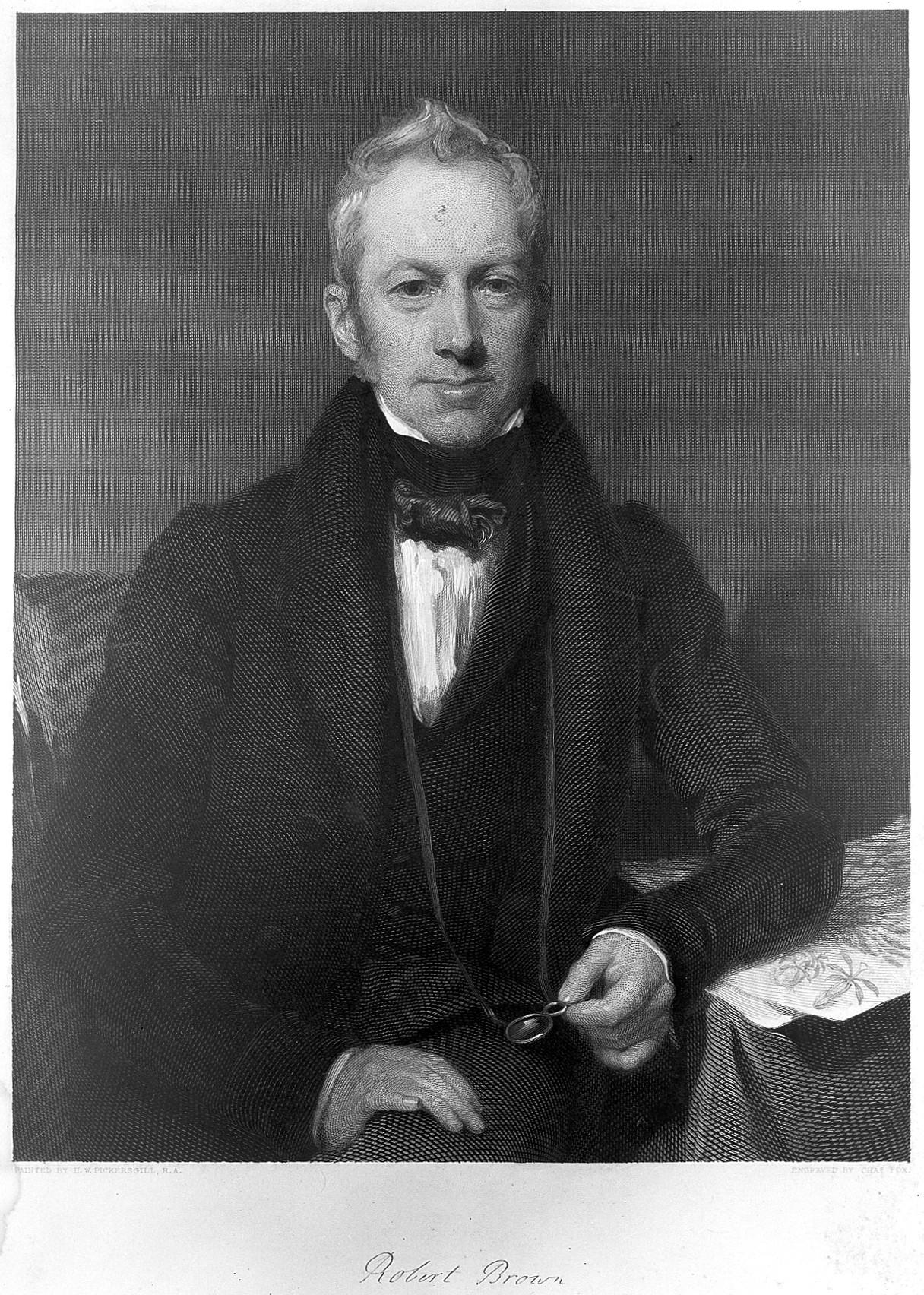
Robert Brown(1773—1858)
A Scottish botanist who took part in botanical exploration in Australia and also studied the microscopic structure of plants.
In 1827, while studying tiny particles in pollen, he observed their persistent, irregular motion in a liquid.
By the early nineteenth century, microscopes already allowed people to observe many structures invisible to the naked eye.
Studying pollen, Brown noticed that very small particles kept trembling and changing position even when suspended in apparently still water.
At first, this motion seemed possibly related to life.
But Brown went on to study particles of nonliving matter and found that similar motion was not confined to living materials.
It could therefore not be attributed simply to the pollen being alive.
Brown made these observations in 1827 and published his report in 1828. Others had observed similar phenomena earlier, so his important contribution was a systematic investigation of the universality of the motion among different small particles, rather than being “the first to see particles move.” 〔31, 32〕
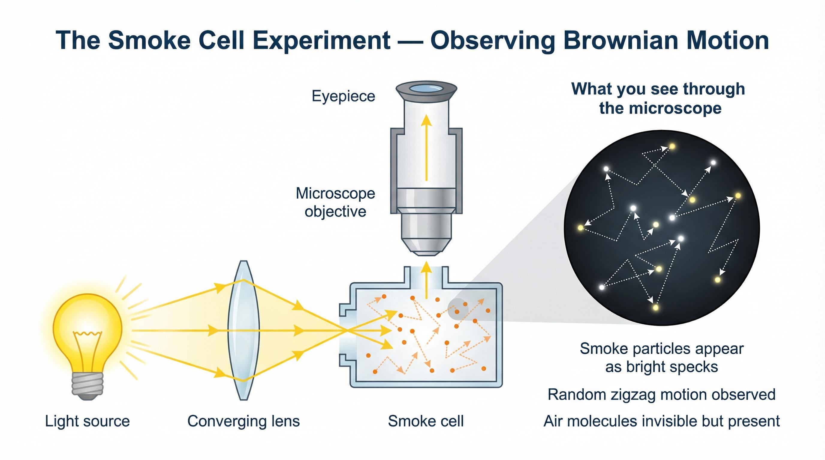
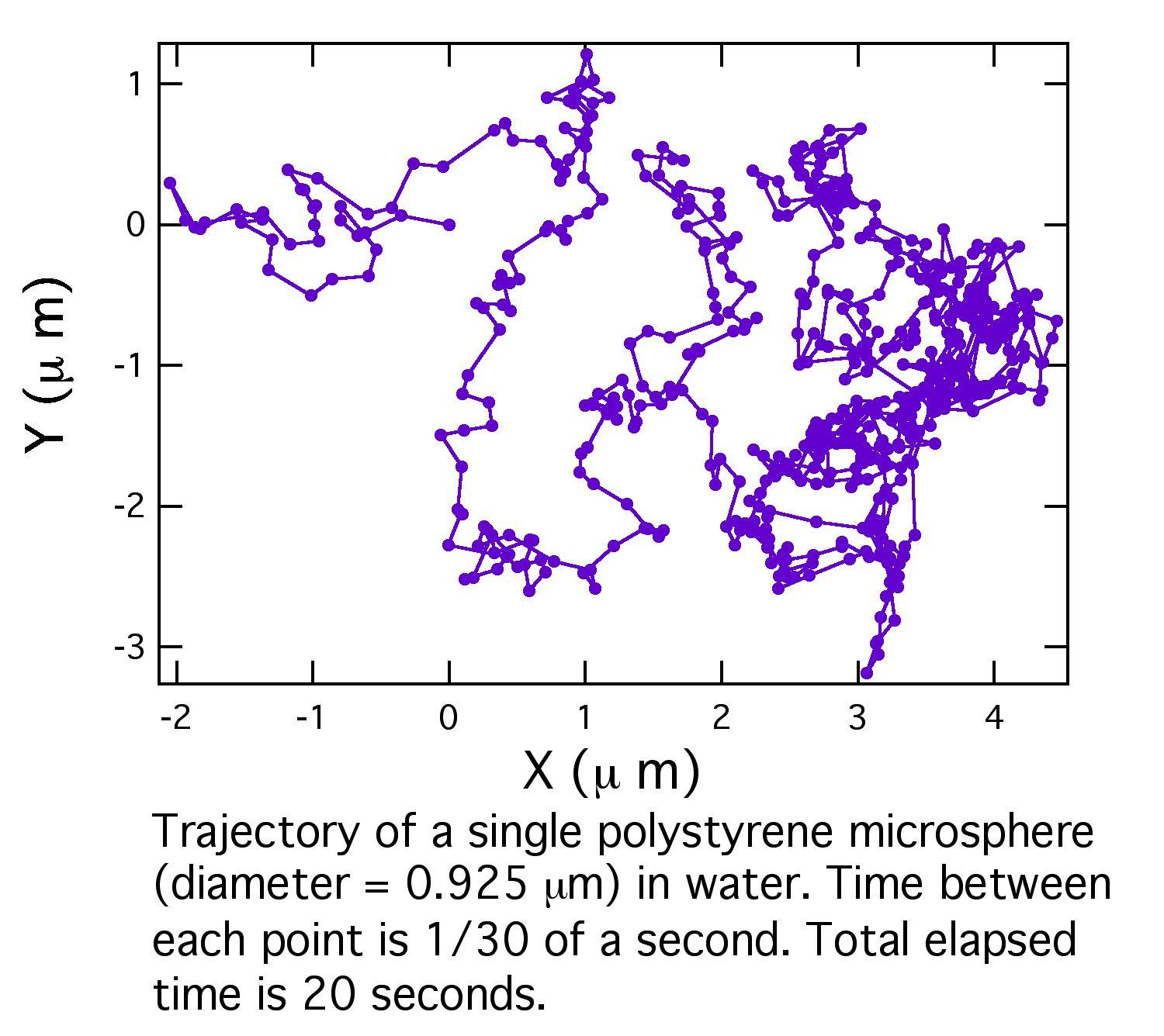
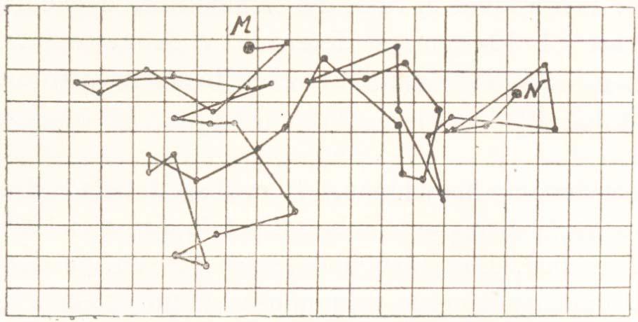
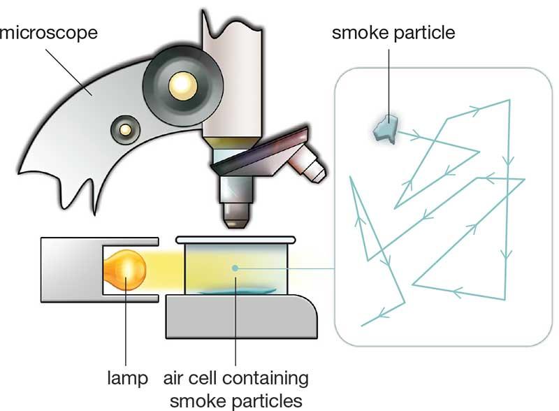

Let us try to think from the perspective of an observer at the time.
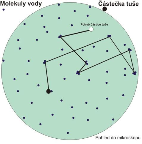
If the water is still and the particle cannot move under its own power, why does it keep moving?
If some invisible microscopic action continually pushes these particles, can countless tiny motions that we cannot directly observe produce statistical laws measurable at a macroscopic scale?
This question later became closely connected with the kinetic theory of molecules, evidence for the existence of atoms, and statistical physics.
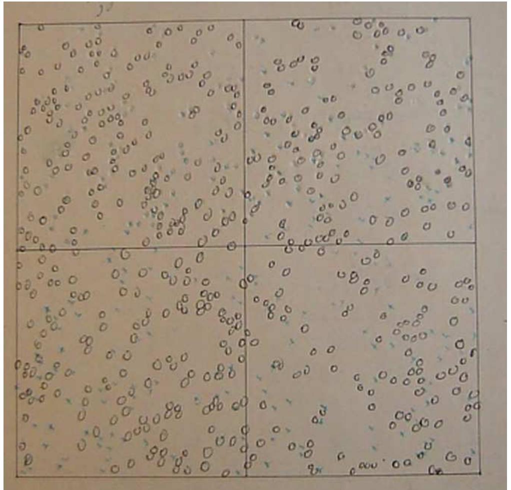
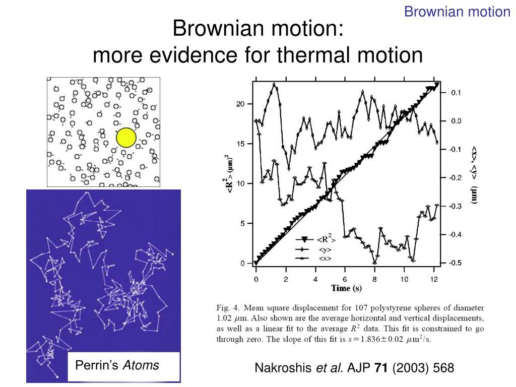
In 1905, Einstein gave a quantitative theory of the diffusion of suspended particles; Smoluchowski proposed a related theory in 1906. Jean Perrin's subsequent experiments provided important support for the predictions. 〔33, 34, 35〕
There is also a historical episode worth noticing.
Before the physical theory of Brownian motion had matured, the French mathematician Louis Bachelier studied a similar continuous random price model in his 1900 financial mathematics thesis Théorie de la spéculation.
The rigorous probabilistic foundations of this continuous stochastic process are closely associated with Norbert Wiener's work in the 1920s, particularly in 1923.
Today, mathematical standard Brownian motion is also called the Wiener process. 〔36, 37〕
But that history came later.
To understand how such a process arises, we must first set aside continuous time, continuous paths, and even the normal distribution.
We begin with the smallest possible model.
4.2 A Particle That Can Move Only Left or Right at Each Step
Imagine a particle on the integer line.
It starts at the origin.
At each unit of time, it randomly moves one unit to the right or left.
Let
\xi_1,\xi_2,\ldotsbe independent, identically distributed random variables with
P(\xi_i=1)=P(\xi_i=-1)=\frac12.Define
S_0=0,\qquad
S_n=\sum_{i=1}^n\xi_i.
Then
S_nis the particle's position after n steps.
This is the one-dimensional simple symmetric random walk.
We already have most of the knowledge needed to study this model.
Since
\mathbb E[\xi_i]=0,
\qquad
\operatorname{Var}(\xi_i)=1,
we have
\boxed{
\mathbb E[S_n]=0,\qquad
\operatorname{Var}(S_n)=n.
}
and hence
\mathbb E[S_n^2]=n.If we measure the typical distance from the origin by the root-mean-square displacement, then
\boxed{
\sqrt{\mathbb E[S_n^2]}=\sqrt n.
}
This is rather strange.
If the particle always moves right, its distance from the origin after n steps is n.
But when independent, symmetric randomness determines its direction, its root-mean-square displacement is only \sqrt n.
Displacement scales for random walks and deterministic motion
The displacement of deterministic motion in one direction is n;the root-mean-square displacement of a symmetric random walk is √n。
查看母稿数值表
| n | Motion always in the same direction | Root-mean-square displacement of a random walk |
|---|---|---|
| 0 | 0 | 0 |
| 1 | 1 | 1 |
| 4 | 4 | 2 |
| 9 | 9 | 3 |
| 16 | 16 | 4 |
| 25 | 25 | 5 |
| 36 | 36 | 6 |
| 49 | 49 | 7 |
| 64 | 64 | 8 |
| 81 | 81 | 9 |
| 100 | 100 | 10 |
The displacement scale of random motion is thus quite different from that of deterministic motion at constant speed.
Motion at constant speed satisfies
x(t)\propto t.In this random-walk model, however, the typical displacement satisfies
|S_n|_{\mathrm{typical}}\propto\sqrt n.Of course, an individual random trajectory may deviate enormously.
\sqrt n is not a deterministic bound that holds for every sample path.
It is first of all a statistical scale supplied by the second moment.
But this scale will become the key to understanding continuous random motion.
4.3 What Becomes of a Random Walk as Time Is Divided More Finely?
Let us pose a thought experiment.
Suppose we no longer want the particle to move once per second.
Instead, let it move n times in one second.
Each move then takes time
\Delta t=\frac1n.At the same time, shrink the spatial length of each step to
\Delta x=\frac1{\sqrt n}.In time t, the particle then takes approximately nt steps.
The variance of its total displacement is therefore approximately
nt\cdot\frac1n=t.This means that
even as individual steps shrink and the number of steps per unit time grows, the total displacement retains a nontrivial variance.
We get neither a completely stationary particle nor a system that diverges infinitely in finite time.
Now define
\boxed{
W_n(t)=\frac{S_{\lfloor nt\rfloor}}{\sqrt n},
\qquad t\ge0.
}
Here \lfloor nt\rfloor denotes the largest integer no greater than nt.
This is the random walk after simultaneous rescaling of time and space.
Let us observe how it changes.
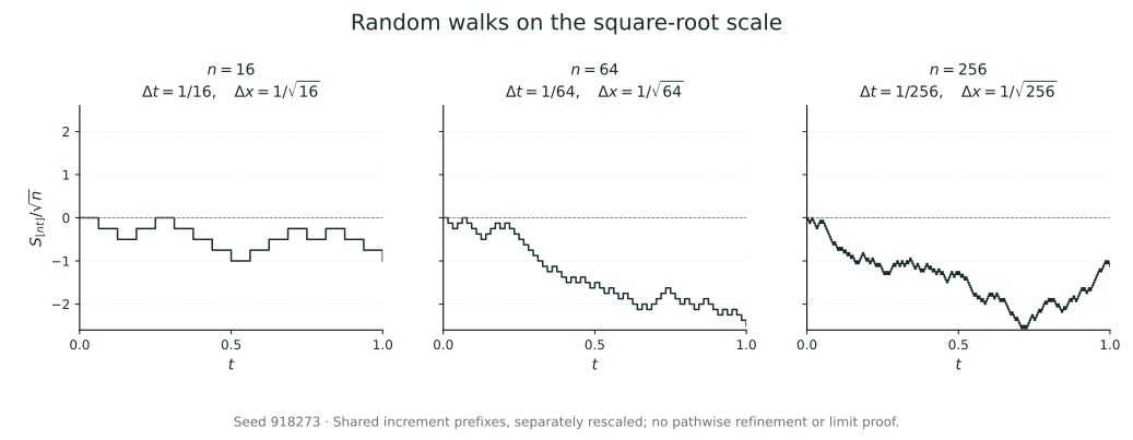
A scaling experiment for discrete random walks. Number of time steps: 16, 32, 64, 128, 256. Illustrative simulation: each step has length 1/\sqrt n and each time interval is 1/n. To aid comparison, different-length prefixes of the same pregenerated sequence of random increments are used; the figure does not rigorously depict successive approximations of one and the same path.
As n increases, the original large jumps become smaller and more densely spaced.
We begin to expect that, in some limiting sense, this process will form a continuous random path.
But this immediately raises two mathematical questions.
First, does such a limit really exist?
Second, even if it exists, in what sense should we understand convergence of an entire random path?
The central limit theorem so far describes only how the distribution of a single random variable converges.
Now we want an entire function to converge:
t\longmapsto W_n(t).This distinction will be crucial.
4.4 Why Must the Spatial Scale Be the Square Root of the Time Scale?
Let us avoid assuming that the scaling exponent is 1/2.
Suppose time is still shrunk by 1/n, but the spatial step is
n^{-\alpha}where \alpha>0.
Define
W_n^{(\alpha)}(t)
=
n^{-\alpha}S_{\lfloor nt\rfloor}.
Since
\operatorname{Var}(S_{\lfloor nt\rfloor})=\lfloor nt\rfloor,we have
\operatorname{Var}(W_n^{(\alpha)}(t))
=
n^{-2\alpha}\lfloor nt\rfloor.
For fixed t>0, the asymptotic scale is
t n^{1-2\alpha}.Three quite different cases arise.
If
\alpha>\frac12,then
\operatorname{Var}(W_n^{(\alpha)}(t))\to0.The random displacement tends to zero in probability, giving a degenerate limit.
If
\alpha=\frac12,then
\operatorname{Var}(W_n^{(\alpha)}(t))\to t.the fluctuations retain a finite, nonzero scale in the limit.
If
\alpha<\frac12,the variance tends to infinity. For this symmetric random walk, the central limit theorem further shows that, for any fixed M>0,
P(|W_n^{(\alpha)}(t)|\le M)\to0.The distributions at a fixed time therefore do not form a tight family of probability distributions on the real line.
Thus only
\boxed{\alpha=\frac12}can give us the nondegenerate diffusion limit we seek.
This choice of scale is profound.
\boxed{
\text{time scale}\sim\varepsilon^2,
\qquad
\text{space scale}\sim\varepsilon.
}
It differs from deterministic motion at constant speed, where
\text{space scale}\sim\text{time scale}.In random diffusion, time and space obey a quadratic relationship.
When we later study scaling limits of random trees, the CRT, and other continuous random geometric objects, we will encounter this idea again:
Finding the right scaling exponent is often the first step toward discovering the limiting object.
The actual exponent, however, depends on the random structure of the model. Not every random system must have the Brownian exponent 1/2.
4.5 The Central Limit Theorem Sees Only One Time
Return to
W_n(t)=\frac{S_{\lfloor nt\rfloor}}{\sqrt n}.First fix a time t>0.
Since
S_{\lfloor nt\rfloor}
=
\xi_1+\cdots+\xi_{\lfloor nt\rfloor},
the central limit theorem gives
\frac{S_{\lfloor nt\rfloor}}{\sqrt{\lfloor nt\rfloor}}
\xrightarrow d N(0,1).
Thus
W_n(t)
=
\frac{S_{\lfloor nt\rfloor}}{\sqrt{\lfloor nt\rfloor}}
\sqrt{\frac{\lfloor nt\rfloor}{n}}.
Since
\frac{\lfloor nt\rfloor}{n}\to t,we obtain
\boxed{
W_n(t)\xrightarrow d N(0,t).
}
If a continuous-time limit exists, we see that its position at each fixed time t should therefore be normally distributed with mean 0 and variance t.
Its density should thus be
\boxed{
p_t(x)
=
\frac1{\sqrt{2\pi t}}
\exp\left(-\frac{x^2}{2t}\right).
}
But notice:
This conclusion describes only a single fixed time.
It says nothing about the relationship between the positions at t=1 and t=2, or where the particle travels between those times.
A stochastic process is much more than a separate probability distribution at each time.
4.5.1 Why Is Knowing the Distribution at Every Time Insufficient?
Consider two stochastic processes.
The first is
X_t=\sqrt t\,Z,where
Z\sim N(0,1).Then, for each t>0,
X_t\sim N(0,t).Temporarily denote the second process by B_t, and require it also to satisfy
B_t\sim N(0,t).The two processes therefore have the same distribution at each fixed time.
For the first process, however,
X_s=\sqrt{\frac st}X_t
\qquad(0<s<t).
Knowing its position at one nonzero time determines its position at every other time.
Its entire path is simply a deterministic function of the form
t\longmapsto \sqrt t\,zwith a random coefficient z.
Consequently,
\operatorname{Cov}(X_s,X_t)=\sqrt{st}.The Brownian motion we seek, however, will satisfy
\operatorname{Cov}(B_s,B_t)=\min(s,t).These are clearly different.
In particular, when 0<s<t,
\sqrt{st}\ne s.Two stochastic processes can thus have exactly the same distribution at every time while having entirely different temporal structures.
To study a stochastic process, we must understand joint distributions across different times, beyond the marginal distribution at each time.
4.5.2 From One Time to Several
Choose times
0=t_0<t_1<\cdots<t_m.We study the random vector
(W_n(t_1),\ldots,W_n(t_m)).The most natural way to understand it is to study the increments between adjacent times rather than each coordinate separately:
\Delta_{n,j}=W_n(t_j)-W_n(t_{j-1}).For the step process defined here, these increments are exactly sums of random steps over distinct time intervals; boundary terms require control only if we switch to the linearly interpolated version (see Appendix F).
For example,
\Delta_{n,j}
=
\frac1{\sqrt n}
\sum_{k=\lfloor nt_{j-1}\rfloor+1}^{\lfloor nt_j\rfloor}\xi_k.
Different intervals use disjoint collections of random variables, so the increments are independent.
Each increment also satisfies the central limit theorem:
\Delta_{n,j}
\xrightarrow d
N(0,t_j-t_{j-1}).
The entire increment vector should therefore converge to a collection of independent normal random variables:
(Z_1,\ldots,Z_m),where
Z_j\sim N(0,t_j-t_{j-1}).Characteristic functions prove this joint convergence rigorously: independence factors the joint characteristic function into a product, and each factor converges to the characteristic function of the corresponding normal distribution.
Then, using
W_n(t_j)=\sum_{r=1}^j\Delta_{n,r},we obtain joint convergence of the finite-dimensional distributions.
We have therefore found the structure that the continuous limit should satisfy:
\boxed{
B_{t_j}-B_{t_{j-1}}
\sim N(0,t_j-t_{j-1}),
}
with independent increments over disjoint time intervals.
This is far stronger than saying that the distribution at every time is normal.
Using characteristic functions to pass from limits of increments to the joint vector limit invokes the multivariate continuity theorem for characteristic functions and preservation of convergence in distribution by continuous linear maps. These will be developed systematically in Chapters 11 and 13, with the language of convergence introduced in Chapter 7. Appendix F retains the product-factorization calculation. This section establishes the finite-dimensional limit conditional on those tools; it does not establish a path limit theorem.
4.5.3 The Covariance Structure Emerges Naturally
From
B_t=B_s+(B_t-B_s),
\qquad s<t,
and independence of increments,
\begin{aligned}
\mathbb E[B_sB_t]
&=\mathbb E[B_s^2]
+\mathbb E[B_s(B_t-B_s)]\\
&=s+0\\
&=s.
\end{aligned}
Thus
\boxed{
\operatorname{Cov}(B_s,B_t)=\min(s,t).
}
We obtain a very special covariance kernel:
\boxed{
K(s,t)=\min(s,t).
}
It encodes the second-order relationships between different times of the entire process in a single function.
More importantly, for a Gaussian process, this covariance kernel together with the mean function determines all finite-dimensional joint distributions.
It appears that we have found the entire finite-dimensional probability structure of Brownian motion.
But a huge logical gap remains.
4.6 Does Knowing All Finite-Dimensional Distributions Mean We Have Constructed a Random Path?
Suppose we know, for every finite collection of times
t_1,\ldots,t_m,the joint distribution that the random vector
(B_{t_1},\ldots,B_{t_m})should have.
Does this already imply that a continuous random path exists,
t\longmapsto B_t?Not necessarily.
Later, under appropriate conditions on the state space, we will use a probability-measure extension theorem to realize consistent finite-dimensional distributions within one stochastic process. Here we first identify the problems a construction must solve, without invoking that theorem in advance to announce that the construction is complete.
Such a construction does not, by itself, automatically guarantee continuous sample paths.
Moreover, even when two processes have the same joint distributions at all finite collections of times, we cannot conclude without qualification that their path properties agree.
This is an easily overlooked trap in moving from random variables to stochastic processes.
4.6.1 A Simple but Decisive Counterexample
Let U\sim\operatorname{Uniform}(0,1) and define
X_t=\mathbf1_{\{t=U\}},
\qquad 0\le t\le1.
For every fixed t,
P(X_t=1)=P(U=t)=0.so
X_t=0\quad\text{a.s.}For any finite collection of deterministic times t_1,\ldots,t_m, we likewise have
P(X_{t_1}=\cdots=X_{t_m}=0)=1.All finite-dimensional distributions of the process (X_t) are therefore exactly the same as those of the identically zero process
Y_t\equiv0in every case.
Yet the complete paths are dramatically different.
For every U\in(0,1), the function
t\longmapsto X_tsuddenly takes the value 1 at t=U and is zero everywhere else.
The path is therefore discontinuous.
The paths of Y_t\equiv0, by contrast, are clearly continuous everywhere.
We even have
\sup_{0\le t\le1}X_t=1
\quad\text{a.s.},
but
\sup_{0\le t\le1}Y_t=0.Notice how far-reaching this is:
\boxed{
\text{all finite-dimensional distributions agree}
\not\implies
\text{path properties agree}.
}
This does not mean finite-dimensional distributions are useless.
On the contrary, they are an essential part of describing a process.
But to study continuous paths, we must also specify the function space in which we construct our random object and explain how fluctuations between different times are controlled.
Otherwise, continuity may be merely a smooth curve drawn on paper, rather than a rigorously established mathematical property.
4.6.2 Another Problem: Finite-Dimensional Convergence Is Not Path Convergence
Even for a sequence of continuous functions, convergence at each fixed time need not imply convergence of the entire path.
For example, consider the functions on [0,1] given by
f_n(t)=\max\left\{1-2n\left|t-\frac1n\right|,0\right\}.As n increases, this triangular spike moves toward 0 and becomes narrower.
For every fixed t\in[0,1],
f_n(t)\to0.But for every sufficiently large n,
\sup_{0\le t\le1}|f_n(t)|=1.Thus these functions do not converge uniformly to the zero function.
This is a very visual warning:
When studying paths, checking what happens at each deterministic time is insufficient. Exceptional fluctuations over increasingly short intervals, increasingly difficult to detect at fixed times, may still prevent convergence of the whole function.
We therefore need a new theory of convergence for stochastic processes. Chapter 7 will first distinguish the various forms of random convergence; later chapters will place these questions in function spaces.
Two obstacles must be distinguished here. Marginal distributions alone do not even describe relationships between times; after all finite-dimensional distributions are known, we must still choose a path space and establish its measurable structure and regularity.
The random spike does not mean that finite-dimensional distributions can never determine the probability law of continuous paths. Once a process is established as a Borel random element in a space of continuous functions, all its finite-dimensional distributions determine its path distribution; proving this requires the measurable structure developed later. The counterexample shows that finite-dimensional information alone cannot establish path continuity without specifying the path space and the version of the process.
Snapshots tell us where a particle appears, but do not automatically provide a random path on which we can discuss “ever reaching” or “remaining throughout.”
This is the chapter's real turning point. The Gaussian limit has not failed; it has brought us to questions it cannot answer on its own.
4.7 The Continuous Random Motion We Seek
After the preceding investigation, we are finally ready for the formal definition.
Definition: Standard Brownian Motion
A real-valued stochastic process
B=(B_t)_{t\ge0}is called a standard Brownian motion if:
1. B_0=0 almost surely;
2. For every 0\le t_0<t_1<\cdots<t_m, the increments
B_{t_1}-B_{t_0},\ldots,B_{t_m}-B_{t_{m-1}}are independent;
3. For every 0\le s<t,
B_t-B_s\sim N(0,t-s);4. Almost every sample path t\mapsto B_t(\omega) is continuous.
The definition no longer seems unexpected.
We discovered each requirement gradually while seeking a continuous limit of random walks.
The first specifies the initial state.
The second preserves the independence of the original random walk over different time intervals.
The third gives the Gaussian increment structure arising from the central limit theorem.
The fourth needs a proof at the level of function spaces; distributions at fixed times alone cannot guarantee it.
These four conditions are requirements on the limiting object, not yet a proof of its existence. In particular, the fourth does not follow automatically from the earlier Gaussian snapshots.
This chapter no longer compresses a rigorous construction into the text immediately after the definition. Later we will separately address how to extend consistent finite-dimensional distributions to a probability measure, how to choose a continuous version, and why entire random-walk paths approach this process. For deeper construction and path-limit questions, see continuous versions and Wiener measure and Donsker and path tightness.
4.8 From Random Walks to the Heat Equation: Why Does Random Motion Produce a Deterministic Partial Differential Equation?
Following the random-walk route, we have identified the requirements Brownian motion should satisfy; its rigorous existence remains to be established later.
Mathematical history offers another important route to the same object:
heat conduction and diffusion.
This connection deserves a careful derivation because it reveals a deep relationship between the random world and deterministic differential equations.
4.8.1 Starting Again from a Discrete Random Walk
Suppose a particle moves on a spatial grid, jumping left or right by \Delta x, with each jump taking time \Delta t.
Let
p(x,t)be the probability mass of the particle at time t at grid point x.
The particle can arrive at x only from its left or right neighbor, so
p(x,t+\Delta t)
=
\frac12p(x-\Delta x,t)
+
\frac12p(x+\Delta x,t).
Rearranging gives
\begin{aligned}
&p(x,t+\Delta t)-p(x,t)\\
&=\frac12\left[
p(x-\Delta x,t)-2p(x,t)+p(x+\Delta x,t)
\right].
\end{aligned}
Divide both sides by \Delta t:
\begin{aligned}
\frac{p(x,t+\Delta t)-p(x,t)}{\Delta t}
=
\frac{(\Delta x)^2}{2\Delta t}
\frac{
p(x-\Delta x,t)-2p(x,t)+p(x+\Delta x,t)
}{(\Delta x)^2}.
\end{aligned}
Now examine this expression.
The left-hand side has the form of a difference quotient in time:
\frac{\partial p}{\partial t}.The right-hand side has the form of a second difference quotient in space:
\frac{\partial^2p}{\partial x^2}.If both grid spacings tend to zero while
\frac{(\Delta x)^2}{2\Delta t}\to D,we formally obtain
\boxed{
\frac{\partial p}{\partial t}
=
D\frac{\partial^2p}{\partial x^2}.
}
This is the one-dimensional diffusion equation, also called the heat equation.
This is a formal derivation of a continuous limit. Rigorously proving that the suitably normalized limit of the discrete probability masses satisfies this partial differential equation requires a local limit theorem, semigroup theory, or other convergence methods. 〔43, 44〕
But it already reveals a mathematical connection that is difficult to overlook:
At the level of probability distributions, a sequence of entirely random tiny movements can produce a deterministic partial differential equation.
4.8.2 Why Is the Heat Equation's Solution Again a Normal Density?
For standard Brownian motion,
B_t\sim N(0,t).so the position density is
p_t(x)=
\frac1{\sqrt{2\pi t}}
e^{-x^2/(2t)}.
Direct partial differentiation verifies that
\boxed{
\frac{\partial p_t}{\partial t}
=
\frac12\frac{\partial^2p_t}{\partial x^2}.
}
For a general diffusion coefficient D, the density is
\boxed{
p_t(x)
=
\frac1{\sqrt{4\pi Dt}}
e^{-x^2/(4Dt)}.
}
Its variance is
\operatorname{Var}(X_t)=2Dt.Thus
\boxed{
\mathbb E[(X_t-X_0)^2]=2Dt
}
holds for a one-dimensional diffusion model starting at the origin with no drift.
This is precisely the mean-square displacement law connecting Einstein's 1905 Brownian motion theory closely with experiment.
Under appropriate physical conditions, the diffusion coefficient can also be related to temperature, fluid viscosity, and particle radius, allowing macroscopically observable random displacements to reveal microscopic properties of matter. 〔35, 31〕
The density obtained from random jumps satisfies a deterministic diffusion equation. For standard Brownian motion, its coefficient is D=1/2; a general D>0 corresponds to the process \sqrt{2D}\,B_t. This explains why we study both the particle's random trajectory and the deterministic evolution of its distribution over time.
Verifying that the Gaussian density satisfies the heat equation does not replace a proof that continuous random paths exist. A density describes the distribution at each time; how a path connects those times remains the open question. For semigroups, generators, and deeper connections to stochastic calculus, continue with semigroups and generators.
4.9 When “It Happened at Some Time” Becomes an Event
If a particle ends up near the origin, can we say it never traveled far?
Of course not. It might have crossed a high horizontal line and then returned. The final position gives only the last snapshot; “having crossed” requires the entire path.
Assume we already have a continuous Brownian path, and ask on [0,1]:
A=\left\{\omega:\sup_{0\le t\le1}B_t(\omega)>1\right\}.This set contains a whole collection of functions with a particular history, rather than a sequence of possible die scores. We want to write P(A), but first must answer: which sets of paths may be assigned probabilities, and why does A belong among them?
Continuity offers a clue. If a continuous path is strictly above 1 at some time, it is also above 1 at a nearby rational time. Thus, for continuous paths,
\left\{\sup_{0\le t\le1}B_t>1\right\}
=\bigcup_{q\in\mathbb Q\cap[0,1]}\{B_q>1\}.
The right-hand side needs only countably many observation times. Here the equality is understood path by path in the continuous path space; if the process is only almost surely continuous, the equality holds on the same probability-one continuity event. Both continuity and the strict inequality matter; the reasoning cannot be applied unconditionally to the earlier random spike. We have not yet used the equality to calculate the probability, but it already indicates which set operations should continue to yield meaningful events when describing entire paths.
Our language must accommodate complements, countable unions, and limits; it must also explain why the maximum of a continuous function can serve as a random quantity. Chapter 5 begins with the sets we may discuss, Chapter 6 develops integration as a language for averaging functions, and Chapter 7 proceeds to different kinds of random convergence. Only then will we be ready to return to Brownian motion and complete the construction and path limits.
Chapter 4 Conclusion: We Know Where the Particle Is, but Not Which Path It Took
Let us return to the microscope.
The particles Brown observed are still moving constantly in the water. Their positions keep changing and their directions seem patternless; even a clear view of a particle's present position cannot predict where it will move next.
To understand this motion, we began with the simplest random walk: each step goes left or right, independently and with equal probability. One step alone cannot reveal the scale of motion over a long period. But when many jumps are combined, cancellations between directions leave a stable scale. Quadrupling the number of steps only doubles the root-mean-square displacement.
As jumps become more frequent and steps become smaller, we therefore cannot rescale time and space arbitrarily. For random motion to persist while retaining a finite scale of fluctuations, we must maintain
\Delta x\sim\sqrt{\Delta t}.At this scale, the Gaussian limit of Chapter 3 reappears: at a fixed time, the particle's position distribution approaches a bell curve whose variance grows with time.
But this gives us only one snapshot.
Collecting separate snapshots at every time does not tell us how the particle moves from one position to another. The same one-time distributions can arise from very different motions. We must turn to joint structure across times and to increments over adjacent time intervals, until independence and Gaussian distributions together give the special covariance kernel:
K(s,t)=\min(s,t).This simple function records the connections between times: the random displacement accumulated at an earlier time becomes part of the later position, while subsequent independent increments bring fresh fluctuations.
When we turn from the trajectory of one particle to the position distribution of many particles, another regularity appears. At the standardized diffusion scale, the Gaussian density satisfies
\frac{\partial p}{\partial t}
=\frac12\frac{\partial^2p}{\partial x^2}.
The irregular motion seen under the microscope connects here with the deterministic heat equation. Individual trajectories are hard to predict, yet the distribution of possible positions can evolve regularly.
Just as we seem to be gradually understanding the motion, however, a more fundamental question emerges.
We know where the particle may be at a given time, but have not yet established its entire continuous random path in a rigorous probability space.
One-time distributions do not determine relationships across time. Even when every finite-dimensional distribution is specified, existence and measurability of continuous paths cannot be skipped. Our definition of Brownian motion describes the properties this motion should possess, but we must still prove that these requirements can be realized together.
In studying motion, we often care about more than the final snapshot. Has the particle ever reached a given height? Can it remain in a region throughout an interval? When does it first reach a given position?
All these questions depend on the entire path. Returning near the origin at the end does not erase the long journey a particle may have made.
The outcome of a random experiment can therefore be an entire function. We want to group paths with the same kind of history and assign a probability to that collection; before writing that probability, we must know why such a set of paths is an event we are allowed to discuss.
The particle brings us back to the question left open in Chapter 1. Counting gave clear answers for finite games of chance. Now the possible outcomes are entire continuous functions, and the old answer is insufficient.
How should probability be defined?
Toward Chapter 5: Why Does Probability Need Measure Theory?
Let us simplify the difficulty. For now, set aside choosing a random path in function space, and ask only how to choose a real number uniformly from the interval [0,1].
We want the probability of an interval to equal its length. Translating a set should preserve its probability, provided it remains within the interval. Combining countably many disjoint events should give a total probability equal to the sum of their probabilities.
These requirements look natural. But can we retain them all while assigning a probability to every subset of [0,1]?
If even all the sets within an interval cannot be measured this way, we have still more reason to determine exactly which sets can be events before assigning probabilities to entire collections of random paths.
The next chapter begins with this ambition and takes us to the point where it becomes impossible. To understand the particle moving ceaselessly in the water, we must first rethink what it means for an event to be measurable.
The Mathematics of Chance · Volume I, Chapter 4 · Reading Candidate with Revised Conclusion, 2026-10-26